1. Chapter 3 – Set Theory

2. 3.1 Sets and Subsets
A set is a well-defined collection of objects. These objects are called elements and are said to be members of the set.
For a set A, we write x  A if x is an element of A; y  A indicated that y is not a member of A.
A set can be designated by listing its elements within set braces, e.g., A = {1, 2, 3, 4, 5}.
Another standard notation for this set provides us with A = {x | x is an integer and 1  x  5}. Here the vertical line | within the set braces is read “such that”. The symbols {x |…} are read “the set of all x such …”. The properties following | help us determine the elements of the set that is being described.

3. Example 3.1: page 128.

4. Example 3.2: page 128.

5. Example 3.2 page 128
From the above example, A and B are examples of finite sets, where C is an infinite set. For any finite set A, |A| denotes the number of elements in A and is referred to as the cardinality, or size, of A, e.g., |A| = 9, |B| = 4.

6. Definition 3.1:
If C, D are sets from a universe U, we say that C is a subset of D and write C  D, or D  C, if every element of C is an element of D. If, in addition, D contains an element that is not in C, then C is called a proper subset of D, and this is denoted by C  D or D  C.
Note: 1) For all sets C, D from a universe U, if C  D, then x [x  C  x  D],
and if x [x  C  x  D], then C  D.
That is, C  D  x [x  C  x  D].
2) For all subsets C, D of U, C  D  C  D.
3) When C, D are finite, CD  |C||D|, and CD  |C|<|D|.

7. Example 3.3: page 129.

8. Example 3.4: page 129.

9. Definition 3.2:
For a given universe U, the sets C and D (taken from U) are said to be equal, and we write C = D, when C  D and D  C.
Note: Some notions from logic: page 130 (line 4 from top).

10. Example page 130.

11. Example 3.5

12. Theorem 3.1: Let A, B, C  U, a) If AB and BC, then AC.
b) If AB and BC, then AC.
c) If AB and BC, then AC.
d) If AB and BC, then AC.

13. Proof of Theorem 3.1

14. Example 3.6: page 131.

15. Definition 3.3:
The null set, or empty set, is the (unique) set containing no elements. It is denoted by  or { }. (Note that ||=0 but {0}. Also, {} because {} is a set with one element, namely, the null set.)

16. Theorem 3.2:
For any universe U, let AU. Then A, and if A, then A.

17. Example 3.7: page 132.

18. Definition 3.4:
If A is a set from universe U, the power set of A, denoted (A), is the collection (or set) of all subsets of A.

19. Example 3.8: page 132.

20. Lemma:
For any finite set A with |A| = n  0, we find that A was 2n subsets and that |(A)| = 2n. For any 0  k  n, there are subsets of size k. Counting the subsets of A according to the number, k, of elements in a subset, we have the combinatorial identity , for n  0.

21. Example 3.9: page 133.

23. Example 3.10

24. Example 3.11: page 135. (Note: )

25. Example 3.13: page 136. (Pascal’s triangle)

27. 3.2 Set Operations and the Laws of Set Theory

28. Definition 3.5: For A, B  U we define the followings:
A  B (the union of A and B) = {x | x  A  x  B }.
A  B (the intersection of A and B) = {x | x  A  x  B }.
A  B (the symmetric difference of A and B) = {x | (xA  xB)  xAB} = {x | xAB  xAB}.
Note: If A, B  U, then A  B, A  B, A  B  U. Consequently, , , and  are closed binary operations on (A), and we may also say that (A) is closed under these (binary) operations.

29. Example 3.14: page 140.

30. Definition 3.6:
Let S, T  U. The sets S and T are called disjoint, or mutually disjoint, when S  T = .

31. Theorem 3.3:
If S, T  U, then S and T are disjoint if and only if S  T = S  T.
proof) proof by contradiction.

32. Definition 3.7:
For a set A  U, the complement of A denote U – A, or , is given by {x | xU  xA}.

33. Example 3.15: page 141.

34. Definition 3.8:
A, B  U, the (relative) complement of A in B, denoted B – A, is given by {x | xB  xA}.

35. Example 3.16: page 141.

36. Theorem 3.4:
For any universe U and any sets A, B  U, the following statements are equivalent:
a) A  B b) A  B = B
c) A  B = A d) B’  A’

37. The Laws of Set Theory: page 142~143.

39. Definition 3.9:
Let s be a (general) statement dealing with the equality of two set expressions. Each such expression may involve one or more occurrences of sets (such as A, , B, , etc.), one or more occurrences of  and U, and only the set operation symbols  and . The dual of s, denoted sd, is obtained from s by replacing (1) each occurrence of  and U (in s) by U and , respectively; and (2) each occurrence of  and  (in s) by  and , respectively.

40. Theorem 3.5: The Principle of Duality.
Let s denote a theorem dealing with the equality of two set expressions (involving only the set operations  and  as described in Definition 3.9). Then sd, the dual of s, is also a theorem.

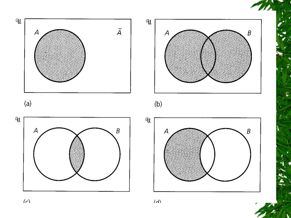
41. Venn diagram
Venn diagram is constructed as follows: U is depicted as the interior of a rectangle, while subsets of U are represented by the interiors of circles and other closed curves. (See Fig 3.5 and 3.6, page 145.)

45. Membership table:
We observe that for sets A, B  U, an element xU satisfies exactly one of the following four situations:
a) xA, xB b) xA, xB
c) xA, xB d) xA, xB.
When x is an element of a given set, we write a 1 in the column representing that set in the membership table; when x is not in the set, we enter a 0. See Table 3.2 and 3.3, page 147.

46. (1) A Venn diagram is simply a graphical representation of a membership table.
(2) The use of Venn diagrams and/or membership tables may be appealing, especially to the reader who presently does not appreciate writing proofs.

47. Example 3.18: page 148.

48. Example 3.19: page 148.

49. Example 3.20

51. Example 3.21

52. Example 3.22

54. 3.3 Counting and Venn Diagrams

56. Fig 3.8 (page 152) demonstrates and , so by the rule of sum, |A| + || = |U| or || = |U| － |A|. If the sets A, B have empty intersection, Fig 3.9 shows |A  B| = |A| + |B|; otherwise, |A  B| = |A| + |B| － | A  B| (Fig 3.10).

57. Lemma: If A and B are finite sets, then
|A  B| = |A| + |B| － | A  B|.
Consequently, finite sets A and B are (mutually) disjoint if and only if |A  B| = |A| + |B|.
In addition, when U is finite, from DeMorgan’s Law we have
|| = || = |U|－|A  B| = |U|－|A|－|B|+|A  B|.

58. Lemma: If A, B, C are finite sets, then .
From the formula for |A  B  C| and DeMorgan’s Law, we find that if the universe U is finite, then
Example 3.25: page 153~154.

59. 3.4 A Word on Probability

60. Lemma:
Under the assumption of equal likelihood, let Φ be a sample space for an experiment Ε. Any subset A of Φ is called an event. Each element of Φ is called an elementary event, so if |Φ| = n and a  Φ, A  Φ, then
Pr(a) = The probability that a occurs =, and
Pr(A) = The probability that A occurs =.

61. Example 3.26: page 154.

62. Example 3.27: page 155.

63. Example 3.29: page 155~156.