2. Random Variables Numerical Quantities whose values are determine by the outcome of a random experiment

3. Discrete Random Variables Discrete Random Variable: A random variable usually assuming an integer value. a discrete random variable assumes values that are isolated points along the real line. That is neighbouring values are not “possible values” for a discrete random variable Note: Usually associated with counting The number of times a head occurs in 10 tosses of a coin The number of auto accidents occurring on a weekend The size of a family

4. Continuous Random Variables Continuous Random Variable: A quantitative random variable that can vary over a continuum A continuous random variable can assume any value along a line interval, including every possible value between any two points on the line Note: Usually associated with a measurement Blood Pressure Weight gain Height

5. Probability Distributions of a Discrete Random Variable

6. Probability Distribution & Function Probability Distribution: A mathematical description of how probabilities are distributed with each of the possible values of a random variable. Notes: The probability distribution allows one to determine probabilities of events related to the values of a random variable. The probability distribution may be presented in the form of a table, chart, formula. Probability Function: A rule that assigns probabilities to the values of the random variable

7. Comments: Every probability function must satisfy: 1.The probability assigned to each value of the random variable must be between 0 and 1, inclusive: 2.The sum of the probabilities assigned to all the values of the random variable must equal 1: 3.

8. Mean and Variance of a Discrete Probability Distribution Describe the center and spread of a probability distribution The mean (denoted by greek letter  (mu)), measures the centre of the distribution. The variance (  2 ) and the standard deviation (  ) measure the spread of the distribution.  is the greek letter for s.

9. Mean of a Discrete Random Variable The mean, , of a discrete random variable x is found by multiplying each possible value of x by its own probability and then adding all the products together: Notes: The mean is a weighted average of the values of X. The mean is the long-run average value of the random variable. The mean is centre of gravity of the probability distribution of the random variable

11.  2 Variance and Standard Deviation Variance of a Discrete Random Variable: Variance,  2, of a discrete random variable x is found by multiplying each possible value of the squared deviation from the mean, (x   ) 2, by its own probability and then adding all the products together: Standard Deviation of a Discrete Random Variable: The positive square root of the variance:

12. Example The number of individuals, X, on base when a home run is hit ranges in value from 0 to 3.

13. Computing the mean: Note: 0.929 is the long-run average value of the random variable 0.929 is the centre of gravity value of the probability distribution of the random variable

14. Computing the variance: Computing the standard deviation:

15. The Binomial distribution 1.We have an experiment with two outcomes – Success(S) and Failure(F). 2.Let p denote the probability of S (Success). 3.In this case q=1-p denotes the probability of Failure(F). 4.This experiment is repeated n times independently. 5.X denote the number of successes occuring in the n repititions.

16. The possible values of X are 0, 1, 2, 3, 4, …, (n – 2), (n – 1), n and p(x) for any of the above values of x is given by: X is said to have the Binomial distribution with parameters n and p.

17. Summary: X is said to have the Binomial distribution with parameters n and p. 1.X is the number of successes occurring in the n repetitions of a Success-Failure Experiment. 2.The probability of success is p. 3. The probability function

18. Example: 1.A coin is tossed n = 5 times. X is the number of heads occurring in the 5 tosses of the coin. In this case p = ½ and x012345 p(x)

19. Note:

21. Computing the summary parameters for the distribution – ,  2, 

22. Computing the mean: Computing the variance: Computing the standard deviation:

23. Example: A surgeon performs a difficult operation n = 10 times. X is the number of times that the operation is a success. The success rate for the operation is 80%. In this case p = 0.80 and X has a Binomial distribution with n = 10 and p = 0.80.

24. Computing p(x) for x = 1, 2, 3, …, 10

25. The Graph

26. Computing the summary parameters for the distribution – ,  2, 

27. Computing the mean: Computing the variance: Computing the standard deviation:

28. Notes The value of many binomial probabilities are found in Tables posted on the Stats 244 site. The value that is tabulated for n = 1, 2, 3, …,20; 25 and various values of p is: Hence The other table, tabulates p(x). Thus when using this table you will have to sum up the values

29. Example Suppose n = 8 and p = 0.70 and we want to compute P[X = 5] = p(5) Table value for n = 8, p = 0.70 and c =5 is 0.448 = P[X  5] P[X = 5] = p(5) = P[X  5] - P[X  4] = 0.448 – 0.194 =.254

30. We can also compute Binomial probabilities using Excel =BINOMDIST(x, n, p, FALSE) The function will compute p(x). =BINOMDIST(c, n, p, TRUE) The function will compute

31. Mean,Variance & Standard Deviation The mean, variance and standard deviation of the binomial distribution can be found by using the following three formulas:

32. Solutions: 1)n = 20, p = 0.75, q = 1 - 0.75 = 0.25  np()(0.)207515  npq()(0. )..2075253751936 Example Example:Find the mean and standard deviation of the binomial distribution when n = 20 and p = 0.75 px x x xx ()(0.) )          20 7525 20 for0, 1, 2,..., 20 2)These values can also be calculated using the probability function:

33. Table of probabilities

34. Computing the mean: Computing the variance: Computing the standard deviation:

35. Histogram  

36. Probability Distributions of Continuous Random Variables

37. Probability Density Function The probability distribution of a continuous random variable is describe by probability density curve f(x).

38. Notes: The Total Area under the probability density curve is 1. The Area under the probability density curve is from a to b is P[a < X < b].

39. Normal Probability Distributions

40. The normal probability distribution is the most important distribution in all of statistics Many continuous random variables have normal or approximately normal distributions

41. The Normal Probability Distribution Points of Inflection

42. Main characteristics of the Normal Distribution Bell Shaped, symmetric Points of inflection on the bell shaped curve are at  –  and  +  That is one standard deviation from the mean Area under the bell shaped curve between  –  and  +  is approximately 2/3. Area under the bell shaped curve between  – 2  and  + 2  is approximately 95%.

43. There are many Normal distributions depending on by  and  Normal  = 100,  = 40Normal  = 140,  =20 Normal  = 100,  =20

44. The Standard Normal Distribution  = 0,  = 1

45. There are infinitely many normal probability distributions (differing in  and  ) Area under the Normal distribution with mean  and standard deviation  can be converted to area under the standard normal distribution If X has a Normal distribution with mean  and standard deviation  than has a standard normal distribution has a standard normal distribution. z is called the standard score (z-score) of X.

46. Example: Suppose a man aged 40-45 is selected at random from a population. X is the Blood Pressure of the man. Assume that X has a Normal distribution with mean  =180 and a standard deviation  = 15. X is random variable.

47. The probability density of X is plotted in the graph below. Suppose that we are interested in the probability that X between 170 and 210.

48. Let Hence

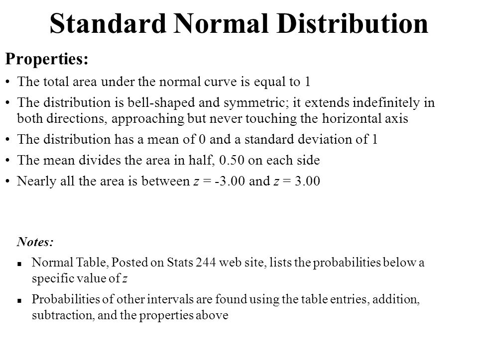
51. Standard Normal Distribution Properties: The total area under the normal curve is equal to 1 The distribution is bell-shaped and symmetric; it extends indefinitely in both directions, approaching but never touching the horizontal axis The distribution has a mean of 0 and a standard deviation of 1 The mean divides the area in half, 0.50 on each side Nearly all the area is between z = -3.00 and z = 3.00 Notes: Normal Table, Posted on Stats 244 web site, lists the probabilities below a specific value of z Probabilities of other intervals are found using the table entries, addition, subtraction, and the properties above

52. Table, Posted on stats 244 web site The table contains the area under the standard normal curve between -  and a specific value of z

53. Example Find the area under the standard normal curve between z = -  and z = 1.45 A portion of Table 3: z0.000.010.020.030.040.050.06 1.40.9265............

54. Pz(0.)  98.01635 Example Find the area to the left of -0.98; P(z < -0.98)

55. Area asked for Example Find the area under the normal curve to the right of z = 1.45; P(z > 1.45)

56. Example Find the area to the between z = 0 and of z = 1.45; P(0 < z < 1.45) Area between two points = differences in two tabled areas

57. Notes Use the fact that the area above zero and the area below zero is 0.5000 the area above zero is 0.5000 When finding normal distribution probabilities, a sketch is always helpful

58. Area asked for Example Example:Find the area between the mean (z = 0) and z = -1.26

59. Example: Find the area between z = -2.30 and z = 1.80

60. Example: Find the area between z = -1.40 and z = -0.50

61. Computing Areas under the general Normal Distributions (mean , standard deviation  ) 1.Convert the random variable, X, to its z-score. Approach: 3.Convert area under the distribution of X to area under the standard normal distribution. 2.Convert the limits on random variable, X, to their z-scores.

62. Example Example:A bottling machine is adjusted to fill bottles with a mean of 32.0 oz of soda and standard deviation of 0.02. Assume the amount of fill is normally distributed and a bottle is selected at random: 1)Find the probability the bottle contains between 32.00 oz and 32.025 oz 2)Find the probability the bottle contains more than 31.97 oz When xz      32.00 32.0 0.00; 0.02   Solutions part 1) When xz      32025 32.0253202532.0 125.;. 0.02.  

63. PXP X Pz (.) 0.. (.). 32.032025 32.0 02 32.0 02 3202532.0 02 012503944              Graphical Illustration:

64. PxP x Pz(.). (....             3197 32.0 0.02 319732.0 0.02 150) 100000066809332 Example, Part 2)