1. 0 Portfolio Managment 3-228-07 Albert Lee Chun Construction of Portfolios: Introduction to Modern Portfolio Theory Lecture 3 16 Sept 2008

2. 1 Course Outline Sessions 1 and 2 : The Institutional Environment Sessions 1 and 2 : The Institutional Environment Sessions 3, 4 and 5: Construction of Portfolios Sessions 3, 4 and 5: Construction of Portfolios Sessions 6 and 7: Capital Asset Pricing Model Sessions 6 and 7: Capital Asset Pricing Model Session 8: Market Efficiency Session 8: Market Efficiency Session 9: Active Portfolio Management Session 9: Active Portfolio Management Session 10: Management of Bond Portfolios Session 10: Management of Bond Portfolios Session 11: Performance Measurement of Managed Portfolios Session 11: Performance Measurement of Managed Portfolios

3. Albert Lee Chun Portfolio Management 2 Portfolio Risk as a Function of the Number of Stocks in the Portfolio 7-2

4. Albert Lee Chun Portfolio Management 3 Portfolio Diversification 7-3

5. Albert Lee Chun Portfolio Management 4 w 1 = proportion of funds in Security 1 w 2 = proportion of funds in Security 2 r 1 = expected return on Security 1 r 2 = expected return on Security 2 Two-Security Portfolio: Return 7-4

6. Albert Lee Chun Portfolio Management 5  1 2 = variance of Security 1  2 2 = variance of Security 2 Cov(r 1,r 2 ) = covariance of returns for Security 1 and Security 2 Two-Security Portfolio: Risk 7-5

7. Albert Lee Chun Portfolio Management 6  1,2 = Correlation coefficient of returns  1 = Standard deviation of returns for Security 1  2 = Standard deviation of returns for Security 2 Covariance 7-6

8. Albert Lee Chun Portfolio Management 7 Range of values for  1,2 + 1.0 >  > -1.0 If  = 1.0, the securities would be perfectly positively correlated If  = - 1.0, the securities would be perfectly negatively correlated Correlation Coefficients: Possible Values 7-7

9. Albert Lee Chun Portfolio Management 8 Three-Security Portfolio 7-8

10. Albert Lee Chun Portfolio Management 9 Generally, for an n-Security Portfolio: 7-9

11. Albert Lee Chun Portfolio Management 10 Review of Portfolio Statistics

12. Albert Lee Chun Portfolio Management 11 Today’s Lecture Utility Functions, Indifference Curves Utility Functions, Indifference Curves Capital Allocation Line Capital Allocation Line Minimum Variance Portfolios Minimum Variance Portfolios Optimal Portfolios in a Optimal Portfolios in a 2 security world (1 risk-free and 1 risky) 2 security world (2 risky) 2 security world (2 risky) 3 security world (2 risky and 1 risk-free) 3 security world (2 risky and 1 risk-free) N security world (with and without risk-free asset) N security world (with and without risk-free asset)

13. Albert Lee Chun Portfolio Management 12 Utility Functions

14. Albert Lee Chun Portfolio Management 13 Risk Aversion Given a choice between two assets with equal rates of return, risk-averse investors will select the asset with the lower level of risk. Given a choice between two assets with equal rates of return, risk-averse investors will select the asset with the lower level of risk. Risk-averse investors need to be compensated for holding risk. Risk-averse investors need to be compensated for holding risk. The higher rate of return on a risky asset i is determined by the risk-premium: The higher rate of return on a risky asset i is determined by the risk-premium: E(Ri) – Rf.

15. Albert Lee Chun Portfolio Management 14 Example: Risk Premium W 2 = $80 Profit = -$20 W 1 = $150 Profit = $50 p =.6 100 Risky Investment T-bills Profit = $5 Expected return: (50%)(.6) + (-20%)(.4) = 22% E(Ri) – Rf Risk Premium = E(Ri) – Rf = 22% - 5% = = 17% 1-p =.4

16. Albert Lee Chun Portfolio Management 15 Measure of Investor Preferences A utility function captures the level of satisfaction or happiness of an investor. A utility function captures the level of satisfaction or happiness of an investor. The higher the utility, the happier the investors. The higher the utility, the happier the investors. For example, if investor utility depends only of the mean (let = E(R)) and variance () of returns then it can be represented as a function: For example, if investor utility depends only of the mean (let µ= E(R)) and variance (  2 ) of returns then it can be represented as a function: The locus of portfolios that provide the same level of utility for an investor defines an indifference curve. The locus of portfolios that provide the same level of utility for an investor defines an indifference curve. U = f ( µ,  )

17. Albert Lee Chun Portfolio Management 16 Example: An Indifference Curve U = 5 The investor is indifferent between X and Y, as well as all points on the curve. All points on the curve have the same level of utility (U=5).  (Rp)

18. Albert Lee Chun Portfolio Management 17 Direction of Increasing Utility Expected Return Standard Deviation Direction of Increasing Utility U1U1 U2U2 U3U3 U3 > U2 > U1

19. Albert Lee Chun Portfolio Management 18 Two Different Investors U3U3 U2U2 U1U1 U 3’ U 2’ U 1’ Expected Return Standard Deviation Which investor is more risk averse?

20. Albert Lee Chun Portfolio Management 19 Quadratic Utility The utility of the investor is quadratic if only the mean and variance of returns is important for the investor. The utility of the investor is quadratic if only the mean and variance of returns is important for the investor. A is a constant that determines the degree of risk aversion: it increases with the risk-aversion of the investor. (Note that the 1/2 is just a normalizing constant.) A is a constant that determines the degree of risk aversion: it increases with the risk-aversion of the investor. (Note that the 1/2 is just a normalizing constant.) Note that A > 0, implies that investors dislike risk. The higher the variance the lower the utility. Note that A > 0, implies that investors dislike risk. The higher the variance the lower the utility.

21. Albert Lee Chun Portfolio Management 20 Indifference Curves Let’s look at an example of points on an indifference curve for an investor with a quadratic utility function. Note that higher variance is accompanied by a higher rate of return to compensate the risk-averse nature of the investor.

22. Albert Lee Chun Portfolio Management 21 Certain Equivalent The certain equivalent is the risk-free (certain) rate of return that offers investors the same level of utility as the risky rate of return. The certain equivalent is the risk-free (certain) rate of return that offers investors the same level of utility as the risky rate of return. The investor is indifferent between a risky return and it’s certain equivalent. The investor is indifferent between a risky return and it’s certain equivalent. Example: Suppose an investor has quadratic utility with A = 2. A risky portfolio offers an E(R) equal to 22% and standard deviation 34%. The utility of this portfolio is: Example: Suppose an investor has quadratic utility with A = 2. A risky portfolio offers an E(R) equal to 22% and standard deviation 34%. The utility of this portfolio is: U = 22% - ½ × 2 × (34%)² = 10.44% U = 22% - ½ × 2 × (34%)² = 10.44% The certain equivalent is equal to 10.44% because the utility of obtaining a certain rate of return of 10.44% is The certain equivalent is equal to 10.44% because the utility of obtaining a certain rate of return of 10.44% is U = 10.44% - ½ × 2 × (0%)² = 10.44% U = 10.44% - ½ × 2 × (0%)² = 10.44%

23. Albert Lee Chun Portfolio Management 22 Risk-Neutral Indifference Curves E(R P ) PP PP U4U4 U4U4 U3U3 U3U3 U2U2 U2U2 U1U1 U1U1 Neutral attitude toward risk. Investor is indifferent between different levels of standard deviation. Neutral attitude toward risk. Investor is indifferent between different levels of standard deviation. U3 > U2 > U1

24. Albert Lee Chun Portfolio Management 23 Slope of the Indifference Curve A steep indifference curve coincides with strong risk- aversion. A steep indifference curve coincides with strong risk- aversion. The slope of the indifference curve captures the required compensation for each unit of additional risk. The slope of the indifference curve captures the required compensation for each unit of additional risk. This compensation is measured in units of expected return for each unit of standard deviation. This compensation is measured in units of expected return for each unit of standard deviation. High risk-aversion implies a high degree of compensation for taking on an additional unit of risk and is represented by a steep slope. High risk-aversion implies a high degree of compensation for taking on an additional unit of risk and is represented by a steep slope.

25. Albert Lee Chun Portfolio Management 24 Risk-Averse Indifference Curves E(R P ) PP PP U4U4 U4U4 U3U3 U3U3 U2U2 U2U2 U1U1 U1U1 Expected Return Standard Deviation U3 > U2 > U1

26. Albert Lee Chun Portfolio Management 25 Two Different Investors U3U3 U2U2 U1U1 U 3’ U 2’ U 1’ Expected Return Standard Deviation Which investor is more risk averse? More risk averse Less risk averse

27. Albert Lee Chun Portfolio Management 26 Stochastic Dominance Prefers any portfolio in Z1 to X. Prefers X to any portfolio in Z4. The rankings between portfolios in Z2 or Z3 and X, depends on the preferences of the investor!

28. Albert Lee Chun Portfolio Management 27 Imagine a world with 1 risk-free security and 1 risky security

29. Albert Lee Chun Portfolio Management 28 1 Risk-Free Asset and 1 Risky Asset Note: The variance of the risk-free asset is 0, and the covariance between a risky asset and a risk free asset is naturally equal to 0. Suppose we construct a portfolio P consisting of 1 risk-free asset f and 1 risky asset A:

30. Albert Lee Chun Portfolio Management 29 1 Risk Free Asset and 1 Risky Asset E (r A ) = 15% r f = 7% 0 A f   P =16.5% E(r P ) = 13% P E( r P ) =.25*.07+.75*15=13%  p =.75*.22 = 16.5% Suppose W A =.75  A =22%

31. Albert Lee Chun Portfolio Management 30 E (r A ) rfrf 0 A f  pp E(r p ) P AA Capital Allocation Line (CAL) Slope of CAL Equation of CAL Line Intercept

32. Albert Lee Chun Portfolio Management 31 Maximize Investor Utility In our world with 1 risk free asset and 1 risky asset, if an investor has quadratic utility, what is the optimal portfolio allocation? In our world with 1 risk free asset and 1 risky asset, if an investor has quadratic utility, what is the optimal portfolio allocation? Utility: Expected return and variance: Goal is to Maximize utility. How?

33. Albert Lee Chun Portfolio Management 32 Normally a Bear Lives in a Cave, that is Concave, then to find the top of the cave (i.e. or to maximize a concave function), take the first derivative and set it equal to 0: A concave function has a negative second derivative.

34. Albert Lee Chun Portfolio Management 33 However, if the Bear is Swimming in a Bowl, that is Convex, Then to find the bottom of the bowl (i.e. or to minimize a convex function), take the first derivative and set equal to 0: A convex function has a positive second derivative.

35. Albert Lee Chun Portfolio Management 34 Maximize Investor Utility Take derivative of U with respect to w and set equal to 0: w* is the optimal weight on risky asset A

36. Albert Lee Chun Portfolio Management 35 Example 1 Supppose E(r A ) = 15%;  (r A ) = 22% and r f = 7% and we have a Quadratic investor with A = 4, then w* = (0.15-0.07)/[4*(0.22) 2 ] w* = (0.15-0.07)/[4*(0.22) 2 ] = 0.41 His optimal allocation is: 41% of his capital in the risky portfolio A and 59% in the risk-free asset. E(r p ) = 0.59*7%+0.41*15%=10.28% and  (r p ) = 0.41*0.22=9.02%

37. Albert Lee Chun Portfolio Management 36 Example 2 Supppose E(r A ) = 15%;  (r A ) = 22% and r f = 7% and we have a less risk-averse Quadratic investor with A = 1, then w* = (0.15-0.07)/[1*(0.22) 2 ] = 1.65 > 1 = 1.65 > 1 This investor should place 165% of his capital in A. He needs to borrow 65% of his capital at the risk free rate of 7%. This investor should place 165% of his capital in A. He needs to borrow 65% of his capital at the risk free rate of 7%. E(R p ) = 1.65(0.15) + -0.65(0.07)= 20.2% E(R p ) = 1.65(0.15) + -0.65(0.07)= 20.2%  (r p ) = 1.65*0.22= 0.363 = 36.3%  (r p ) = 1.65*0.22= 0.363 = 36.3% His utility is: U = 0.202 – 0.5*1*(0.363 2 ) = 0.1361

38. Albert Lee Chun Portfolio Management 37 Graphical View A E(r)  7% Ex1: Lender Ex2: Borrower  A = 22% The optimal allocation along the capital allocation line depends on the risk-aversion of the agent. Risk-seeking agents with w* greater than 1 will borrow at the risk-free rate and invest in security A The optimal allocation is the point of tangency between the CAL and the investor’s utility function.

39. Albert Lee Chun Portfolio Management 38 Different Borrowing Rate What if the borrowing rate is higher than the lending rate? What if the borrowing rate is higher than the lending rate? E(r)  9% 7% A  A = 22% w* = (0.15-0.09)/[1*(0.22) 2 ] = 1.24 1.24 < 1.65

40. Albert Lee Chun Portfolio Management 39 Different Borrowing Rate Supppose E(r A ) = 15%;  (r A ) = 22% and r f = 7% lending rate, and a 9% borrowing rate, Quadratic investor with A = 1, then w* = (0.15-0.09)/[1*(0.22)2] = 1.24 1.24 < 1.65 This investor should place 124% of his capital in A. He needs to borrow 24% of his capital at the risk free rate of 9%. This is less than what he would borrow at a 7% borrowing rate. This investor should place 124% of his capital in A. He needs to borrow 24% of his capital at the risk free rate of 9%. This is less than what he would borrow at a 7% borrowing rate. E(R p ) = 1.24(0.15) + -0.24(0.09)= 16.44% E(R p ) = 1.24(0.15) + -0.24(0.09)= 16.44%  (r p ) = 1.24*0.22= 27.28%  (r p ) = 1.24*0.22= 27.28% Increasing the borrowing rate, lowers his utility from before: U = 0.1644 – 0.5*1*(0.2728 2 ) =.1272 <.1361

41. Albert Lee Chun Portfolio Management 40 Imagine a world with 2 risky securities

42. Albert Lee Chun Portfolio Management 41 Expected Return and Standard Deviation with Various Correlation Coefficients 7-41

43. Albert Lee Chun Portfolio Management 42 Portfolio Expected Return as a Function of Investment Proportions 7-42

44. Albert Lee Chun Portfolio Management 43 Portfolio Standard Deviation as a Function of Investment Proportions 7-43

45. Albert Lee Chun Portfolio Management 44 Returning to the Two-Security Portfolio and, or Question: What happens if we use various securities’ combinations, i.e. if we vary  ? 7-44

46. Albert Lee Chun Portfolio Management 45 Portfolio Expected Return as a function of Standard Deviation 7-45

47. Albert Lee Chun Portfolio Management 46 Perfect Correlation E(R) R ij = +1.00 D E With two perfectly correlated securities, all portfolios will lie on a straight line between the two assets. With short selling

48. Albert Lee Chun Portfolio Management 47 Perfect Correlation  = +1

49. Albert Lee Chun Portfolio Management 48 Zero Correlation f E(R) R ij = 0.00 R ij = +1.00 f g h i j k 1 2 With uncorrelated assets it is possible to create a two asset portfolio with lower risk than either asset!

50. Albert Lee Chun Portfolio Management 49 Zero Correlation  = 0

51. Albert Lee Chun Portfolio Management 50 Positive Correlation E(R) R ij = 0.00 R ij = +1.00 R ij = +0.50 f g h i j k 1 2 With positively correlated assets a two asset portfolio lies between the first two curves

52. Albert Lee Chun Portfolio Management 51 Negative Correlation E(R) R ij = 0.00 R ij = +1.00 R ij = -0.50 R ij = +0.50 f g h i j k 1 2 With negatively correlated assets it is possible to create a portfolio with much lower risk. Negative

53. Albert Lee Chun Portfolio Management 52 Perfect Negative Correlation E(R) R ij = 0.00 R ij = +1.00 R ij = -1.00 R ij = +0.50 f g h i j k 1 2 With perfectly negatively correlated assets it is possible to create a two asset portfolio with NO RISK. How?

54. Albert Lee Chun Portfolio Management 53 Perfect Negative Correlation  = -1 To get a zero- variance portfolio we need to set:

55. Albert Lee Chun Portfolio Management 54 Minimum Variance Portfolio

56. Albert Lee Chun Portfolio Management 55 Minimum Variance Portfolio

57. Albert Lee Chun Portfolio Management 56 Minimum Variance Portfolio 1>  > -1  = -1  = 0  = 1 If no short sales, then MVP is equal to the asset with the minimum variance.* (Our formula doesn’t work here, why? Think about the bear in a cave/bowl.) *With short sales can obtain 0 variance.

58. Albert Lee Chun Portfolio Management 57 Relationship depends on correlation coefficient Relationship depends on correlation coefficient -1.0 <  < +1.0 -1.0 <  < +1.0 The more negative the correlation, the greater the risk reduction potential The more negative the correlation, the greater the risk reduction potential If  = +1.0, no risk reduction is possible (absent short sales). If  = +1.0, no risk reduction is possible (absent short sales). Portfolio of Two Securities: Correlation Effects 7-57

59. Albert Lee Chun Portfolio Management 58 Example: MVP  Example: :  Example: Suppose there are 2 securities A an B: AB  A,B E(r)10%14% 0.2 15%20%  Find the minimum variance portfolio?

60. Albert Lee Chun Portfolio Management 59 Example: MVP

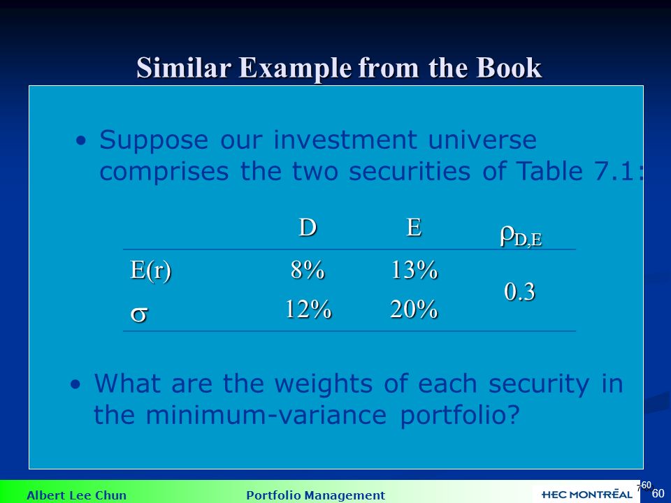
61. Albert Lee Chun Portfolio Management 60 Similar Example from the Book Suppose our investment universe comprises the two securities of Table 7.1: DE  D,E E(r)8%13% 0.3 12%20% What are the weights of each security in the minimum-variance portfolio? 7-60

62. Albert Lee Chun Portfolio Management 61 Book Example: MVP Solving the minimization problem we get: Numerically: 7-61

63. Albert Lee Chun Portfolio Management 62 Investor’s Utility E(r)   More Risk Averse Investors More Risk Averse Investors U’ U’’ U’’’ Less Risk Averse Investors Less Risk Averse Investors

64. Albert Lee Chun Portfolio Management 63 Investor’s Utility Maximization Homework, you should be able to show that the optimal solution is:

65. Albert Lee Chun Portfolio Management 64 Example  Example: :  Example: Suppose there are only 2 portfolios: AB  A,B E(r)10%14% 0.2 15%20%  Find the optimal portfolio for a investor with quadratic utility ( A = 3)?

66. Albert Lee Chun Portfolio Management 65 Example

67. Albert Lee Chun Portfolio Management 66 Imagine a world with 2 risky securities and 1 risk-free security

68. Albert Lee Chun Portfolio Management 67 Two Feasible CALs 7-67

69. Albert Lee Chun Portfolio Management 68 Optimal CAL and the Optimal Risky Portfolio 7-68

70. Albert Lee Chun Portfolio Management 69 With a Risk Free Asset E(r)   CAL 1 CAL 2 CAL 3 I’m the optimal risky portfolio, the tangent portfolio!! I’m the optimal risky portfolio, the tangent portfolio!! I’m the one that maximizes the slope of the Capital Allocation Line ! E E D rfrfrfrf

71. Albert Lee Chun Portfolio Management 70 Optimal Portfolio Weights Homework: If you are ambitious, try to show that the optimal solution is:

72. Albert Lee Chun Portfolio Management 71 The Optimal Overall Portfolio 7-71

73. Albert Lee Chun Portfolio Management 72 The Proportions of the Optimal Overall Portfolio 7-72

74. Albert Lee Chun Portfolio Management 73 Optimal Overall Portfolio: 2 Investors i and j PTPT E(r) rfrf i j CAL  Optimal weight for each investor depends on risk aversion parameter A

75. Albert Lee Chun Portfolio Management 74 Different Lending and Borrowing   E(r) rfrf rfrf P1P1 P1P1 P2P2 P2P2

76. Albert Lee Chun Portfolio Management 75 Now imagine a world with many risky assets

77. Albert Lee Chun Portfolio Management 76 The Markowitz Problem Subject to the constraint

78. Albert Lee Chun Portfolio Management 77 Efficient Frontier E(R)

79. Albert Lee Chun Portfolio Management 78 The optimal combinations result in lowest level of risk for a given return The optimal combinations result in lowest level of risk for a given return The optimal trade-off is described as the efficient frontier The optimal trade-off is described as the efficient frontier These portfolios are dominant These portfolios are dominant Extending Concepts to All Securities 7-78

80. Albert Lee Chun Portfolio Management 79 Minimum Variance Frontier of Risky Assets E(r) Minimum variance frontier Global minimum variance portfolio Individual assets  7-79

81. Albert Lee Chun Portfolio Management 80 Efficient Variance Frontier of Risky Assets E(r) Efficient frontier Global minimum variance portfolio Individual assets  7-80

82. Albert Lee Chun Portfolio Management 81 The Efficient Portfolio Set 7-81

83. Albert Lee Chun Portfolio Management 82 Now imagine a world with many risky assets and 1 risk-free asset

84. Albert Lee Chun Portfolio Management 83 Capital Allocation Lines 7-83

85. Albert Lee Chun Portfolio Management 84 The Market Portfolio Capital Market Line E(R) M

86. Albert Lee Chun Portfolio Management 85 Readings Readings for Today’s lecture. Readings for Today’s lecture. 1. Chapter 7. 1. Chapter 7. 2. If you have not taken Investments, you may want to review Chapter 6 as well. 2. If you have not taken Investments, you may want to review Chapter 6 as well. Readings for next week: Readings for next week: Finish reading Chapter 7, including appedicies. Finish reading Chapter 7, including appedicies. Readings for the week after next: Readings for the week after next: (Course Reader) Other Portfolio Selection Models (Course Reader) Other Portfolio Selection Models