1. Predicting the Present
With Google Trends
Hyunyoung Choi
Hal Varian
June 2009

2. Problem statement
Government agencies and other organizations produce monthly reports on economic activity
Retail Sales
House Sales
Automotive Sales
Unemployment
Problems with reports
Compilation delay of several weeks
Subsequent revisions
Sample size may be small
Not available at all geographic levels
Google Trends releases daily and weekly index of search queries by industry vertical
Real time data
No revisions (but some sampling variation)‏
Large samples
Available by country, state and city
Can Google Trends data help predict current economic activity?
Before release of preliminary statistics
Before release of final revision 2 2

3. Categories in Google Trends by Query Shares
Clearings
Sectors
We have 30 top categories and under the 30 categories, we have 274 subcategories and we have 4 layers of categories with 753 verticals.
Context
This market map shows the top 2 layers of categories – area represents the relative query volume and the color represent the relative growth rate over the year.
From this map, we see that Entertainment categories have high search volume and it’s been growing more than other sectors such as real estate and travel.
For all 753 verticals, we could see the search volume changes over time and depending on the sector of your interest, this data could give some insight on the customer behavior.
Transition
Let’s look at the example of Real estate. As we all know, real estate sector hasn’t been doing that well this year, and you can see it from the color of that sector.
Note: Queries from to & Growth Comparison w/ the same time window 3 3

4. Real Estate

5. Geography
Time window
Category
Clearings
Context
Transition 5 5

6. Subcategories under Real Estate by Query Shares
Real Estate Agencies
Rental Listings & Referrals
Home Insurance
Home Inspections & Appraisal
Property Management
Home Financing
Subcategories under Real Estate by Query Shares 6 6

7. Search on Real Estate Agencies7 7

8. Searches on Rental Listings & Referrals8 8

9. Improving predictions
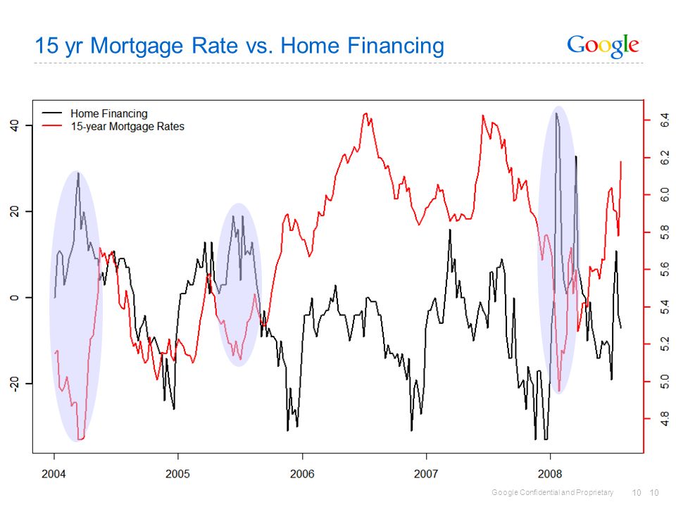
Depicting trends
Google Trends measures normalized query share of particular category of queries – controls for overall growth
Often useful to look at year-on-year changes to eliminate seasonality.
Illustrate correlations and covariates.
Improving predictions
Forecast time series using its own lagged values and add Trends data as a predictor.
Statistical significance?
Improved fit?
Improved forecasts?
Identify turning points? 9 9

10. 15 yr Mortgage Rate vs. Home Financing10 10

11. Forecasting primer Basic forecasting models
Autoregressive: value at time t depends on
Value at time t-1
Seasonal adjustment: value at time t depends on
Value at time t-12
For monthly data
Transfer function: value at time t depends on
Other contemporaneous or lagging variables
Seasonal autoregressive transfer model: Value at time t depends on
Value at time t-12 (seasonality)‏
Value at time t-1 (recent behavior)‏
Other lagging or contemporaneous variables (such as Google Trends data)‏
Typical question of interest
How much more accurate forecasts can you get from additional variables over and above the accuracy you get with the history of the time series itself? 11 11 11 11

12. Model New Home Sales Recent Trend with New Home Sales at t-1
Seasonality with New Home Sales at t-12
Time Series
Exogenous Variables
Housing affordability with Average/Median Home Price
Recent Search Activity on
Real Estate Agencies
Rental Listings & Referrals
Home Inspections & Appraisal
Property Management
Home Insurance
Home Financing
Google Trends

13. Predicting the present
New Residential Sales from US Census
Google Trends Real Estate by Category
Monthly release 24 – 28 days after the month
Seasonally adjusted
National and Regional aggregate
Home Inspections & Appraisal
Home Insurance
Home Financing
Property Management
Rental Listings & Referrals
Real Estate Agencies 13 13

14. New House Sales vs. Real Estate Google Trends
Get new pics
Plot --- Mortgage rate vs. Home financing 14 14

15. Analysis and Forecasting
Model:
Yt = * Yt - 1 – * us * us96.2 – * AvgPt – 1
Yt : New house sold at t-th month
AvgPt – 1: Average Sales Price of New One-Family Houses Sold at (t-1)-th month
us378.1 : Google Trend of vertical id = 378 (Rental Listings & Referrals ) at t-th month 1st week
us96.2 : Google Trend of vertical id = 96 (Real Estate Agent) at t-th month 2nd week
July 2008
Actual = 515K
Predicted = K
Z-score = 2.53
August 2008 Prediction = K 15 15

16. Analysis and Forecasting
Observations
Since 2005 new house sales have been decreasing, with little seasonality
Google Trends captures seasonality & recent trends
Positive association with Real Estate Agencies (96)
Negative association with Rental Listings & Referrals (378) and Average Price 16 16

17. Travel

18. Subcategories under Travel by Query Shares
Hotels & Accommodations
Attractions & Activities
Air Travel
Bus & Rail
Cruises & Charters
Adventure Travel
Car Rental & Taxi Services
Vacation Destinations
Subcategories under Travel by Query Shares 18 18

19. Travel to Hong Kong Hong Kong
Visitors Arrival Statistics from Hong Kong Tourism Board
Google Trends Travel by Category
Monthly summaries release with 1 month lag
Reports Country/Territory of Residence of visitors
Data available
Hotels & Accommodations
Air Travel
Car Rental & Taxi Services
Cruises & Charters
Attractions & Activities
Vacation Destinations
Australia
Caribbean Islands
Hawaii
Hong Kong
Las Vegas
Mexico
New York City
Orlando
Adventure Travel
Bus & Rail 19 19

20. Visitors Arrival Statistics vs. Google Trends20 20

21. Analysis and Forecasting
Model:
log(Yi,t) = * log(Yi,t-1) * log(Yi,t-12) * Xi,t, * Xi,t,3
* FXrate i,t + ηi, + ei,t
ei,t ~ N(0, ), ηi ~ N(0, )‏
Yi,t = Arrival to Hong Kong at month t and from i-th country
Xi,t,1 = Google Trend Search at 1st week of month t and from i-th country
Xi,t,2 = Google Trend Search at 2nd week of month t and from i-th country
Xi,t,3 = Google Trend Search at 3rd week of month t and from i-th country
FXrate i,t = Hong Kong Dollar per one unit of i-th country’s local currency at month t. Average of first week’s FX rate is used as a proxy to FX rate per each month. 21 21

22. Visitor Arrival Statistics - Actual & Fitted22 22

23. Analysis and Forecasting
Conclusion
Arrival at time t is positively associated with arrival at time t-1 and arrival at time t-12.
It shows strong seasonality and autocorrelation
Arrival at time t is positively associated with searches on [Hong Kong].
Arrival at time t is positively associated with FX rates.
When the local currency appreciates relative to Hong Kong Dollar, visitors to Hong Kong increase. 23 23

24. Automobiles

25. Google Trends under Vehicle Brands Category
US Auto Sales by Make
US Auto Sales by Make
Google Trends under Vehicle Brands Category
Monthly summaries released 1 week after end of month
Data available by Car Sales, Truck Sales and Total Sales for each make
Data available from
Source: Automotive News Data Center
Google Trends subcategory Vehicle Brands.
Weekly Search query index
Total 31 verticals in this subcategory
27 verticals matching to Monthly Sales available 25 25 25 25

26. Google Categories under Vehicle Brands
NOTE: Area represents the queries volume from first half year 2008 and the color represents queries yearly growth rate 26 26

27. Auto Sales by Make (Top 9 Make by Sales) Monthly Sales vs
Auto Sales by Make (Top 9 Make by Sales) Monthly Sales vs. Google Trends at Second Week of each month 27 27 27 27

28. Analysis and Forecasting
Fixed effects model:
log(Yi,t) = * log(Yi,t-1) * log(Yi,t-12)
* Xi,t, * Xi,t,2 + ai * Makei + ei,t
ei,t ~ N(0, ) , Adjusted R2 =
Yi,t = Auto Sales of i-th Make at month t
Xi,t,1 = Google Trend Search at 1st week of month t and from i-th make
Xi,t,2 = Google Trend Search at 2nd week of month t and from i-th make
Makei =Dummy variable for Auto Make
ai = Coefficient to capture the mean level of Auto Sales by Make
ANOVA Table
Df Sum Sq Mean Sq F value Pr(>F)
trends < 2e-16 ***
trends
log(s1) < 2e-16 ***
log(s12) < 2e-16 ***
as.factor(brand) < 2e-16 ***
Residuals 28 28 28 28

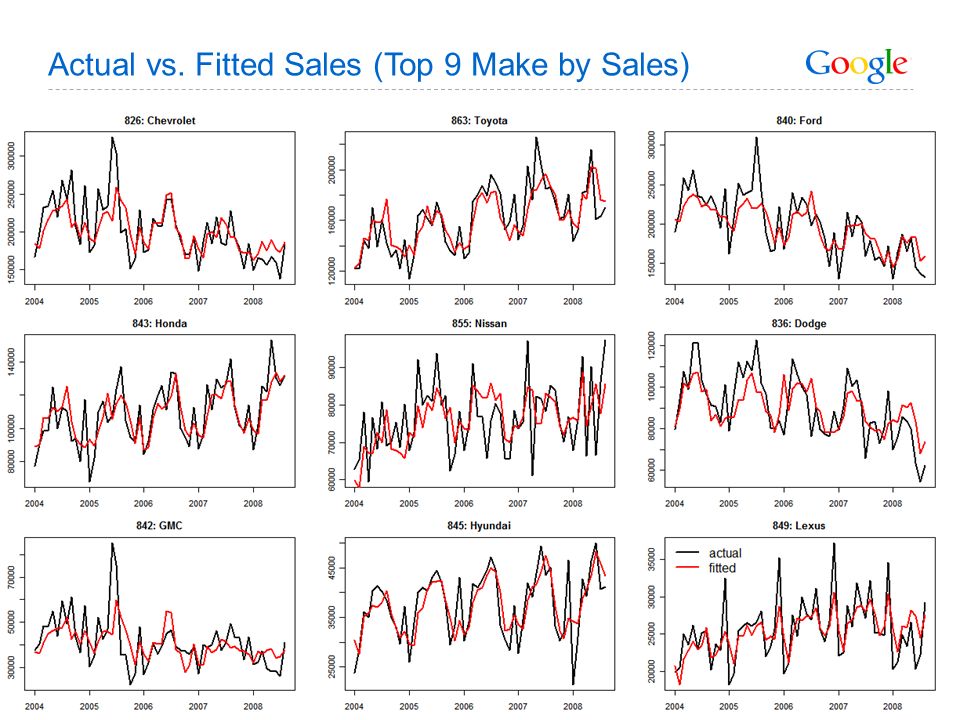
29. Actual vs. Fitted Sales (Top 9 Make by Sales)‏29 29

30. Analysis and Forecasting
Conclusion
Sales at time t are positively associated with Sales at time t-1 and Sales at time t-12.
Sales show strong seasonality and autocorrelation
Monthly Sales are positively correlated to the first and second weeks search volume of each month.
If the search volume increase by 1%, the sales volume will increase by an average of 0.19%. 30 30 30 30

31. Unemployment

32. YoY Growth in Initial Claims & Google Search
According to the NBER, the current recession started December 2007.
National unemployment rate passed 5% in mid 2008 and search queries on [Welfare and Unemployment] also increased at same time.

33. Initial claims is an important leading indicator

34. Google Trends data [Search Insights screenshot]

35. Initial Claims and Google Trends

36. Strong Autocorrelation in Initial Claims
Time Series
Autocorrelation Function

37. Initial Claims Before/After Recession Started
California
New York

38. Time Window for Analysis
Recession Starts
Window For Long Term Model
Window For Short Term Model

39. Model Reference ARIMA(0,1,1) X (1,0,0)12 Model
ARIMA(0,1,1) X (1,0,0)12 Model With Google Trends
Signif. codes: ‘***’ 0.05 ‘**’ 0.01 ‘*’
Model Fit improved significantly – smaller Standard deviation, high log likelihood and smaller AIC
Initial Claims are positively correlated with searches on Jobs and Welfare.

40. Long Term Model: Prediction Comparison with MAE
With Google Trends, the out-of-sample prediction MAE decreases by 16.84%.
Prediction with rolling window from 1/11/2009 to 4/12/2009
Prediction Error at t:
Mean Absolute Error:

41. Short Term Model: Prediction Comparison with MAE
With Google Trends, the out-of-sample prediction MAE decreases by 19.23%.
Prediction errors are within the same range as LT Model.
Fit improvement is better with ST Model.

42. Summary
Google Trends significantly improves out-of-sample prediction of state unemployment, up to 18 days in advance of data release.
Mean absolute error for out-of-sample predictions declines by 16.84% for LT Model and % for ST Model.
Further work
Can examine metro level data
Other local data (real estate)‏
Combine with other predictors
Detect turning points?