1. (C) 2010 Pearson Education, Inc. All rights reserved. Java How to Program, 8/e

2. (C) 2010 Pearson Education, Inc. All rights reserved.

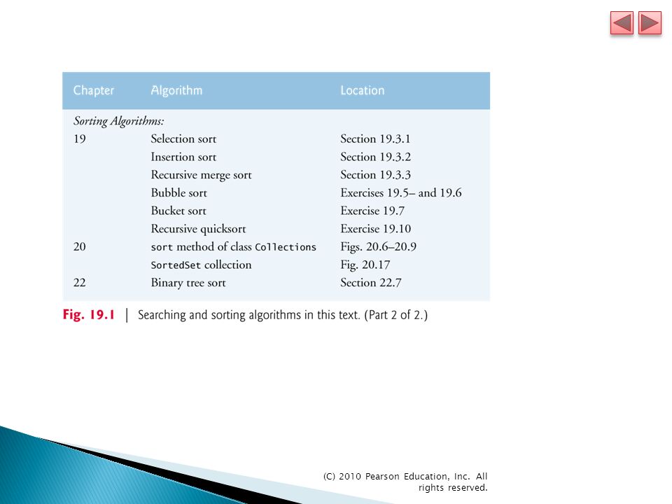
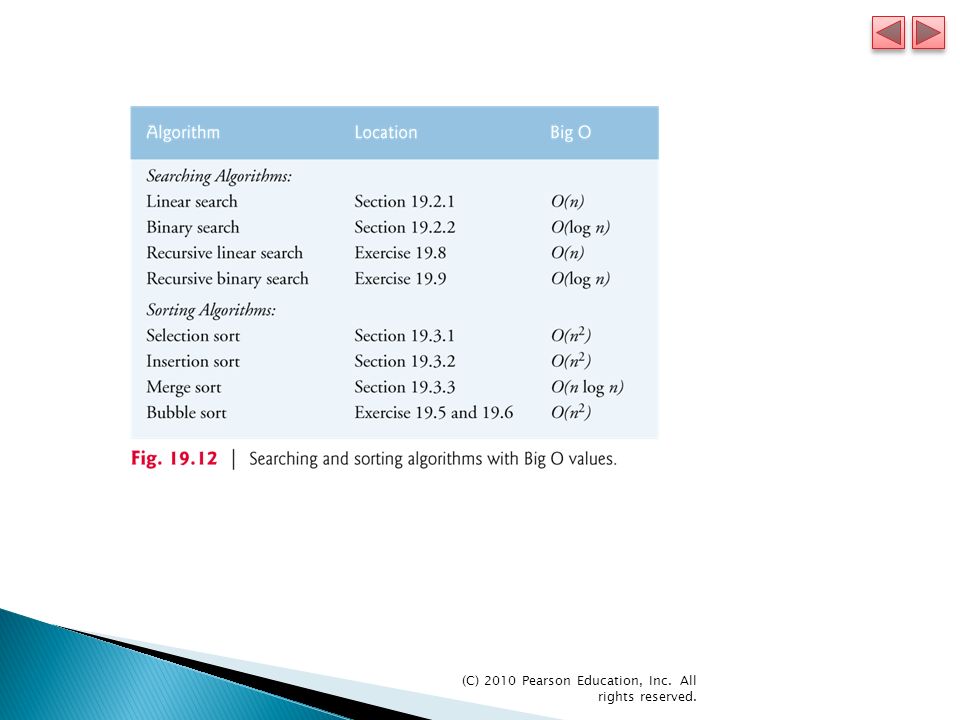
4.  Searching data involves determining whether a value (referred to as the search key) is present in the data and, if so, finding its location. ◦ Two popular search algorithms are the simple linear search and the faster but more complex binary search.  Sorting places data in ascending or descending order, based on one or more sort keys. ◦ This chapter introduces two simple sorting algorithms, the selection sort and the insertion sort, along with the more efficient but more complex merge sort.  Figure 19.1 summarizes the searching and sorting algorithms discussed in the examples and exercises of this book.

5. (C) 2010 Pearson Education, Inc. All rights reserved.

7.  The next two subsections discuss two common search algorithms—one that is easy to program yet relatively inefficient and one that is relatively efficient but more complex and difficult to program.

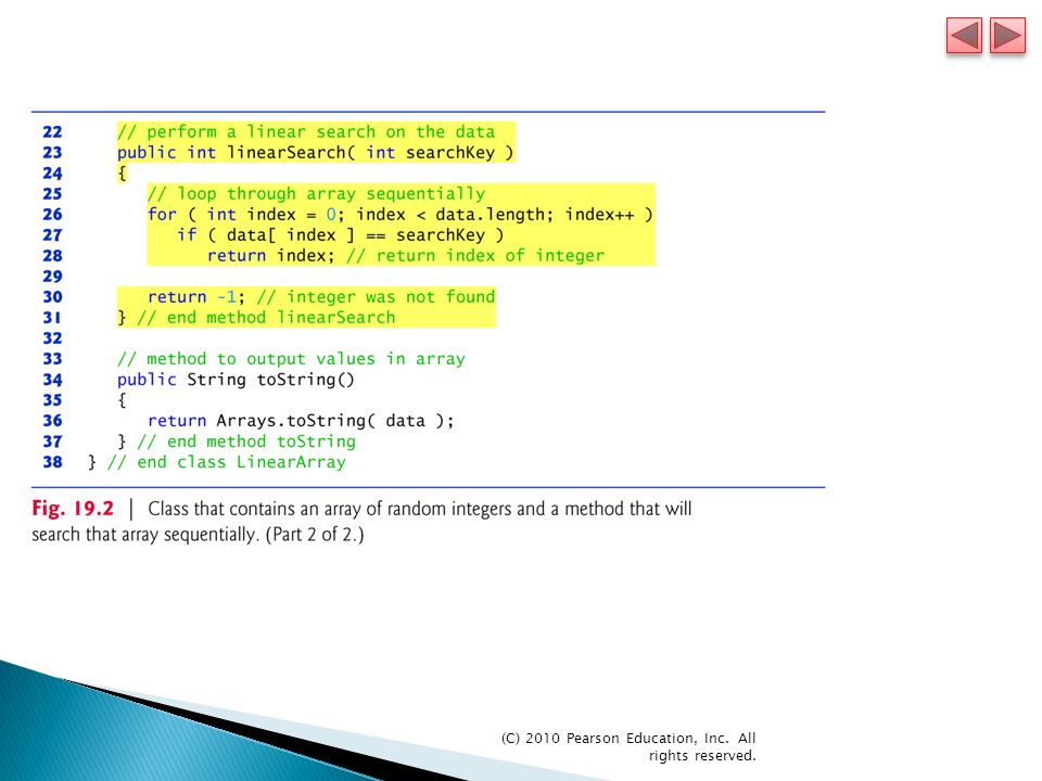
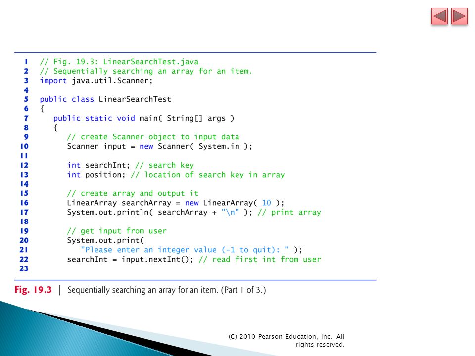
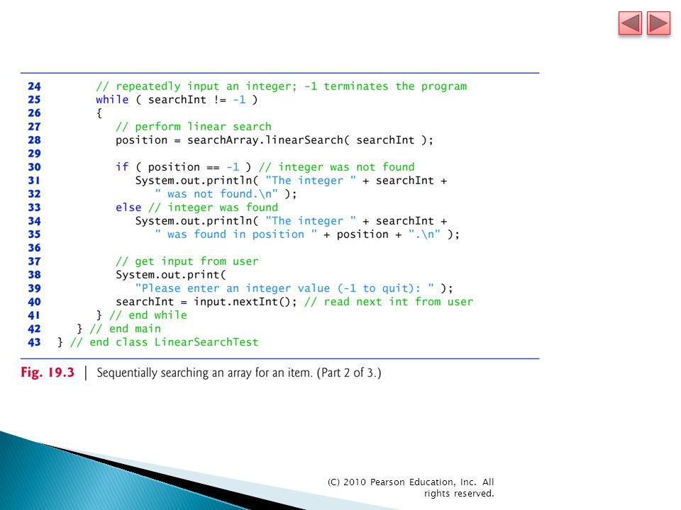
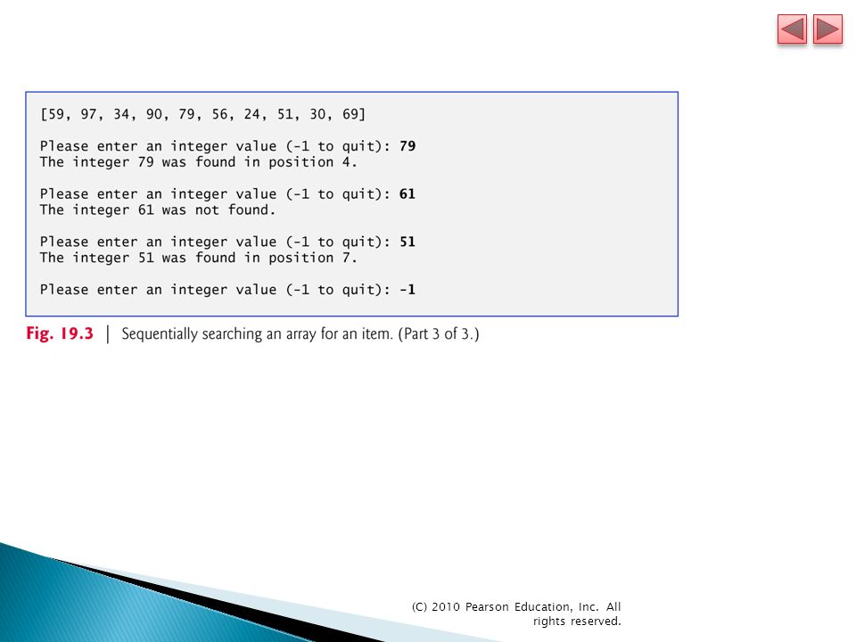
8. (C) 2010 Pearson Education, Inc. All rights reserved.  The linear search algorithm searches each element in an array sequentially. ◦ If the search key does not match an element in the array, the algorithm tests each element, and when the end of the array is reached, informs the user that the search key is not present. ◦ If the search key is in the array, the algorithm tests each element until it finds one that matches the search key and returns the index of that element.  If there are duplicate values in the array, linear search returns the index of the first element in the array that matches the search key.  Arrays static method toString returna a String representation of an array.

9. (C) 2010 Pearson Education, Inc. All rights reserved.

14.  Searching algorithms all accomplish the same goal— finding an element that matches a given search key, if such an element does, in fact, exist.  The major difference is the amount of effort they require to complete the search.  Big O notation indicates the worst-case run time for an algorithm—that is, how hard an algorithm may have to work to solve a problem. ◦ For searching and sorting algorithms, this depends particularly on how many data elements there are.

15. (C) 2010 Pearson Education, Inc. All rights reserved.  If an algorithm is completely independent of the number of elements in the array, it is said to have a constant run time, which is represented in Big O notation as O(1). ◦ An algorithm that is O(1) does not necessarily require only one comparison. ◦ O(1) just means that the number of comparisons is constant—it does not grow as the size of the array increases.  An algorithm that requires a total of n – 1 comparisons is said to be O(n). ◦ An O(n) algorithm is referred to as having a linear run time. ◦ O(n) is often pronounced “on the order of n” or simply “order n.”

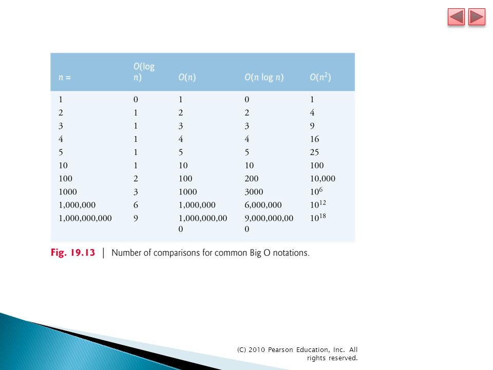
16. (C) 2010 Pearson Education, Inc. All rights reserved.  Constant factors are omitted in Big O notation.  Big O is concerned with how an algorithm’s run time grows in relation to the number of items processed.  O(n 2 ) is referred to as quadratic run time and pronounced “on the order of n-squared” or more simply “order n- squared.” ◦ When n is small, O(n 2 ) algorithms (running on today’s computers) will not noticeably affect performance. ◦ But as n grows, you’ll start to notice the performance degradation. ◦ An O(n 2 ) algorithm running on a million-element array would require a trillion “operations” (where each could actually require several machine instructions to execute). ◦ A billion-element array would require a quintillion operations.  You’ll also see algorithms with more favorable Big O measures.

17. (C) 2010 Pearson Education, Inc. All rights reserved.  The linear search algorithm runs in O(n) time. ◦ The worst case in this algorithm is that every element must be checked to determine whether the search item exists in the array. ◦ If the size of the array is doubled, the number of comparisons that the algorithm must perform is also doubled.  Linear search can provide outstanding performance if the element matching the search key happens to be at or near the front of the array. ◦ We seek algorithms that perform well, on average, across all searches, including those where the element matching the search key is near the end of the array.  If a program needs to perform many searches on large arrays, it’s better to implement a more efficient algorithm, such as the binary search.

18. (C) 2010 Pearson Education, Inc. All rights reserved.

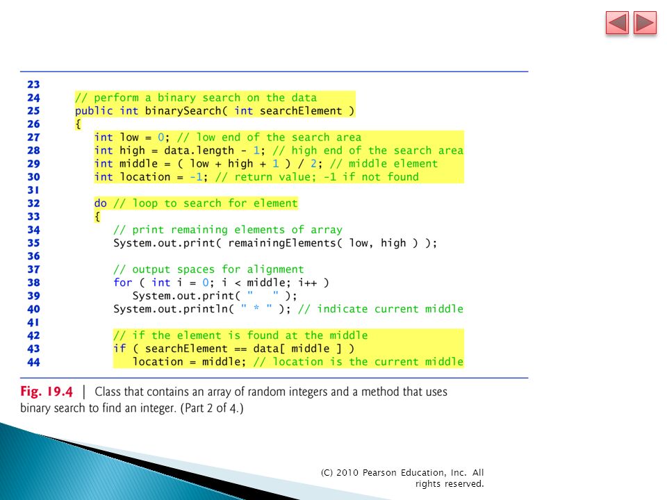
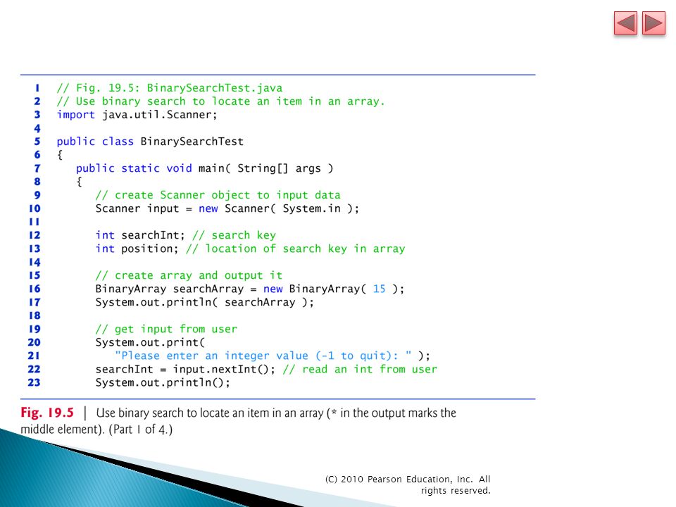
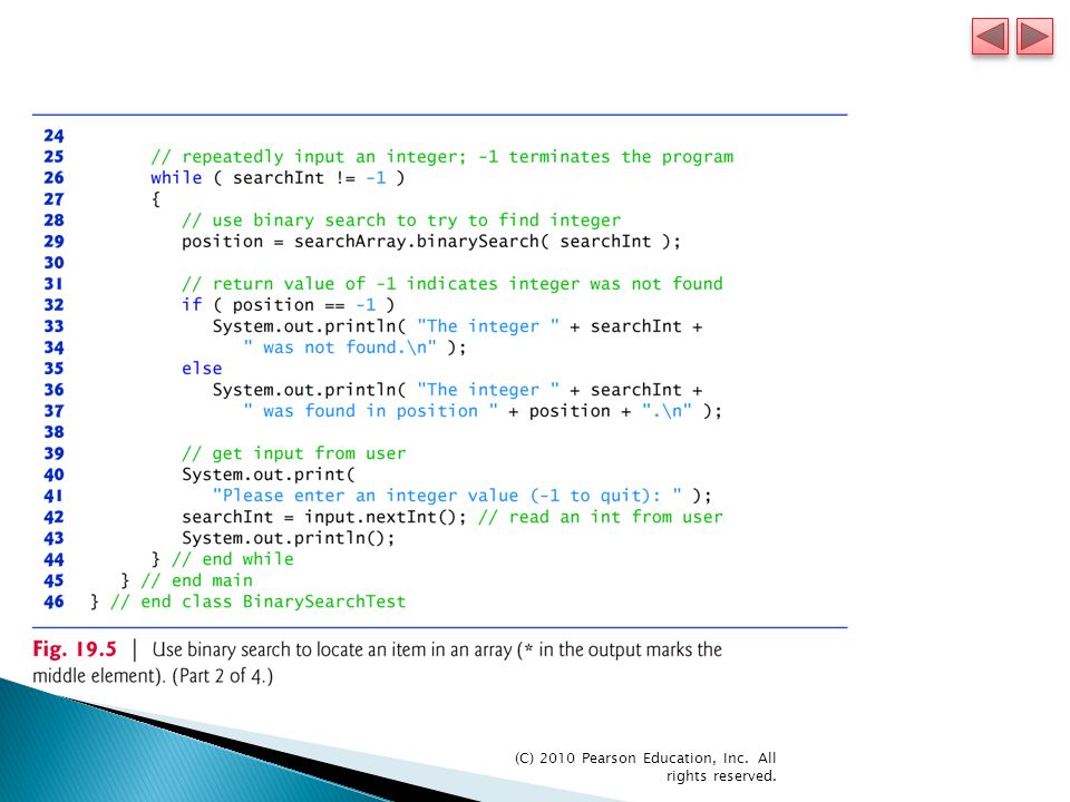
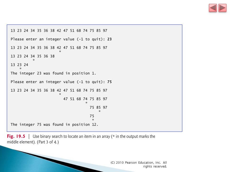
19.  The binary search algorithm is more efficient than linear search, but it requires that the array be sorted. ◦ The first iteration tests the middle element in the array. If this matches the search key, the algorithm ends. ◦ If the search key is less than the middle element, the algorithm continues with only the first half of the array. ◦ If the search key is greater than the middle element, the algorithm continues with only the second half. ◦ Each iteration tests the middle value of the remaining portion of the array. ◦ If the search key does not match the element, the algorithm eliminates half of the remaining elements. ◦ The algorithm ends by either finding an element that matches the search key or reducing the subarray to zero size.

20. (C) 2010 Pearson Education, Inc. All rights reserved.  The sort method is a static method of class Arrays that sorts the elements in an array in ascending order by default; an overloaded version of this method allows you to change the sorting order.

21. (C) 2010 Pearson Education, Inc. All rights reserved.

29.  In the worst-case scenario, searching a sorted array of 1023 elements takes only 10 comparisons when using a binary search. ◦ The number 1023 (2 10 – 1) is divided by 2 only 10 times to get the value 0, which indicates that there are no more elements to test. ◦ Dividing by 2 is equivalent to one comparison in the binary search algorithm.  Thus, an array of 1,048,575 (2 20 – 1) elements takes a maximum of 20 comparisons to find the key, and an array of over one billion elements takes a maximum of 30 comparisons to find the key. ◦ A difference between an average of 500 million comparisons for the linear search and a maximum of only 30 comparisons for the binary search!

30. (C) 2010 Pearson Education, Inc. All rights reserved.  The maximum number of comparisons needed for the binary search of any sorted array is the exponent of the first power of 2 greater than the number of elements in the array, which is represented as log 2 n.  All logarithms grow at roughly the same rate, so in big O notation the base can be omitted.  This results in a big O of O(log n) for a binary search, which is also known as logarithmic run time.

31. (C) 2010 Pearson Education, Inc. All rights reserved.  Sorting data (i.e., placing the data into some particular order, such as ascending or descending) is one of the most important computing applications.  An important item to understand about sorting is that the end result—the sorted array—will be the same no matter which algorithm you use to sort the array.  The choice of algorithm affects only the run time and memory use of the program.  The rest of this chapter introduces three common sorting algorithms. ◦ The first two—selection sort and insertion sort—are easy to program but inefficient. ◦ The last algorithm—merge sort—is much faster than selection sort and insertion sort but harder to program.

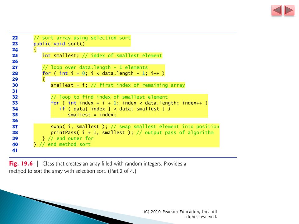
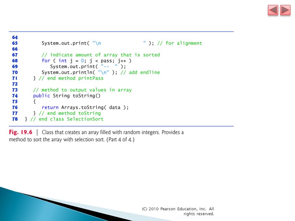
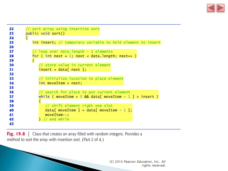
32. (C) 2010 Pearson Education, Inc. All rights reserved.  Selection sort ◦ simple, but inefficient, sorting algorithm  Its first iteration selects the smallest element in the array and swaps it with the first element.  The second iteration selects the second-smallest item (which is the smallest item of the remaining elements) and swaps it with the second element.  The algorithm continues until the last iteration selects the second- largest element and swaps it with the second-to-last index, leaving the largest element in the last index.  After the ith iteration, the smallest i items of the array will be sorted into increasing order in the first i elements of the array.  After the first iteration, the smallest element is in the first position. After the second iteration, the two smallest elements are in order in the first two positions, etc.  The selection sort algorithm runs in O(n 2 ) time.

33. (C) 2010 Pearson Education, Inc. All rights reserved.

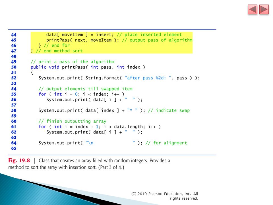
40.  Insertion sort ◦ another simple, but inefficient, sorting algorithm  The first iteration takes the second element in the array and, if it’s less than the first element, swaps it with the first element.  The second iteration looks at the third element and inserts it into the correct position with respect to the first two, so all three elements are in order.  At the ith iteration of this algorithm, the first i elements in the original array will be sorted.  The insertion sort algorithm also runs in O(n 2 ) time.

41. (C) 2010 Pearson Education, Inc. All rights reserved.

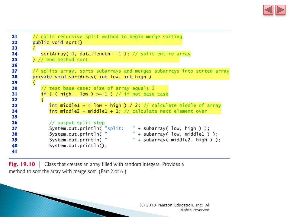
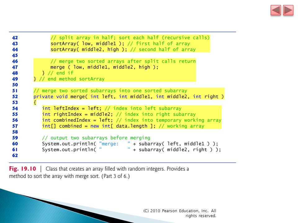
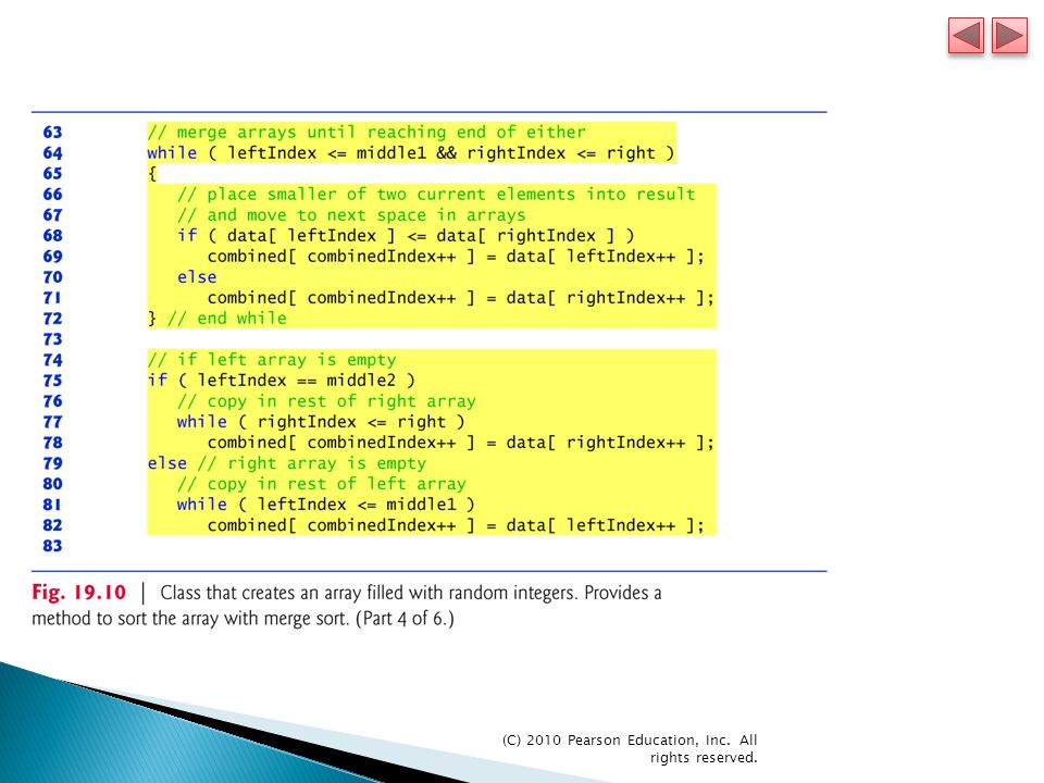
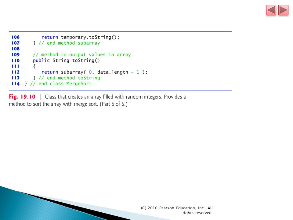
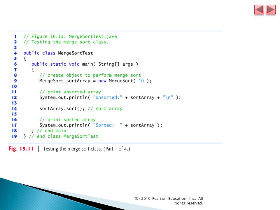
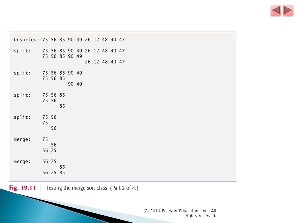
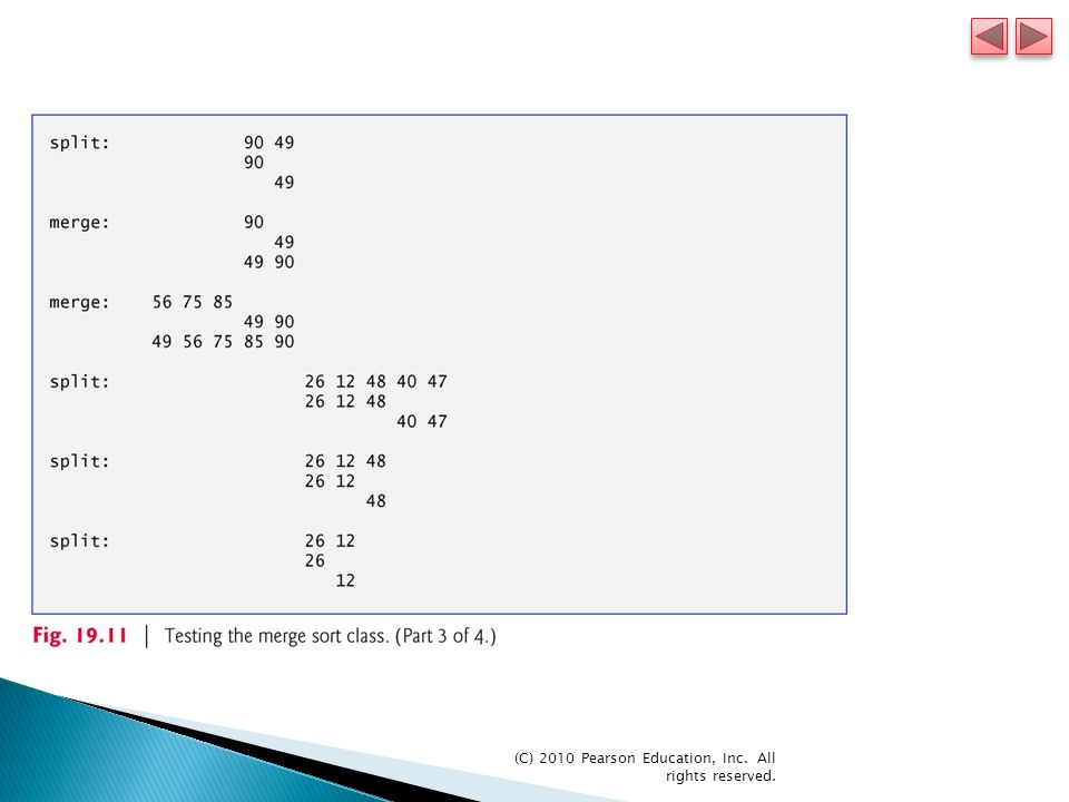
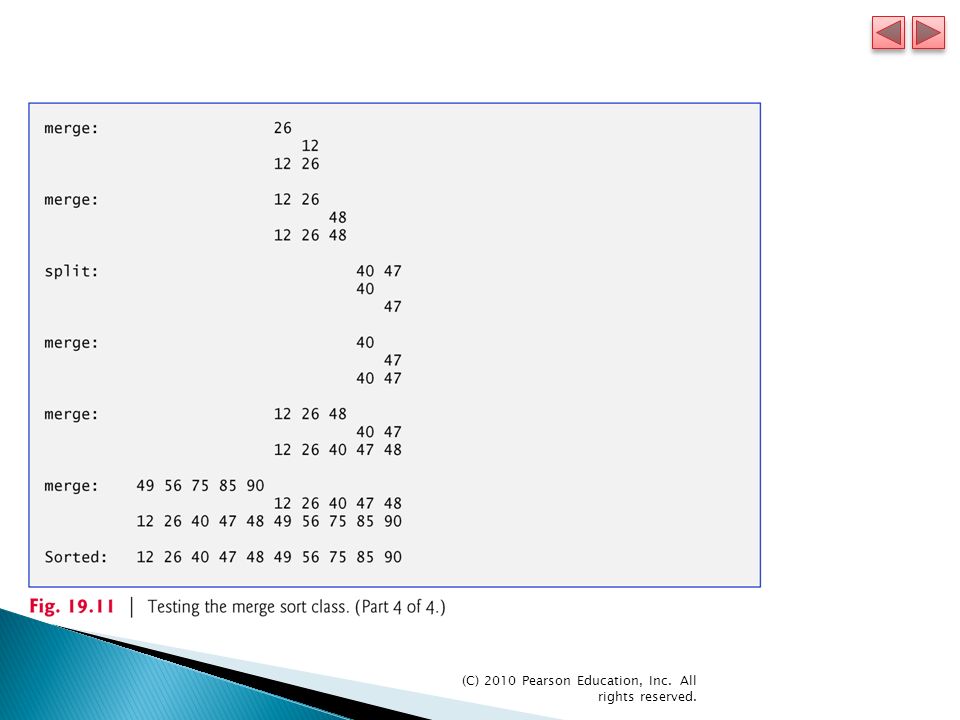
48.  Merge sort ◦ efficient sorting algorithm ◦ conceptually more complex than selection sort and insertion sort  Sorts an array by splitting it into two equal-sized subarrays, sorting each subarray, then merging them into one larger array.  The implementation of merge sort in this example is recursive. ◦ The base case is an array with one element, which is, of course, sorted, so the merge sort immediately returns in this case. ◦ The recursion step splits the array into two approximately equal pieces, recursively sorts them, then merges the two sorted arrays into one larger, sorted array.  Merge sort has an efficiency of O(n log n).

49. (C) 2010 Pearson Education, Inc. All rights reserved.