Download presentation
Presentation is loading. Please wait.

17
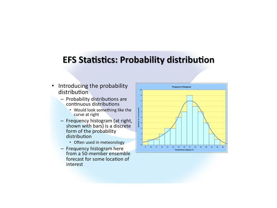
Rank Histograms – measuring the reliability of an ensemble forecast You cannot verify an ensemble forecast with a single observation. The more data you have for verification, (as is true in general for other statistical measures) the more certain you are. Rare events (low probability) require more data to verify => as do systems with many ensemble members. From Barb Brown
 the more certain you are. Rare events (low probability) require more data to verify => as do systems with many ensemble members. From Barb Brown.")
18
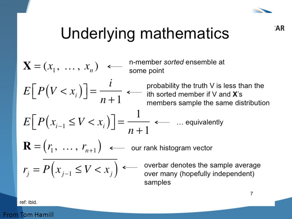
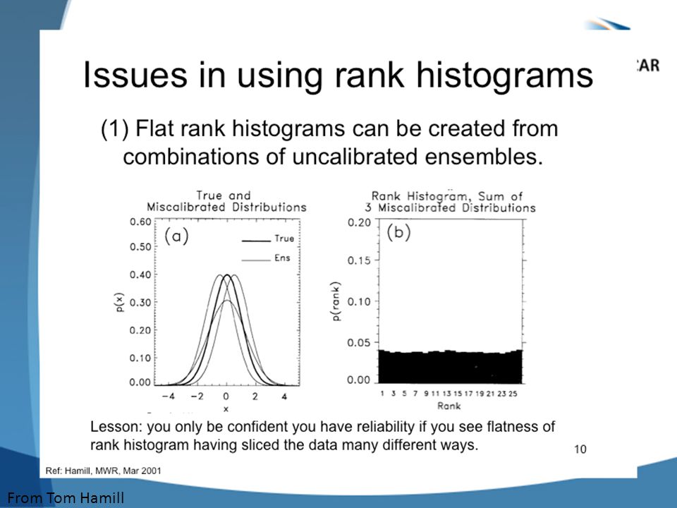
From Tom Hamill

19
Troubled Rank Histograms Slide from Matt Pocernic 1 2 3 4 5 6 7 8 9 10 Ensemble # 1 2 3 4 5 6 7 8 9 10 Ensemble # Counts 0102030 Counts 0102030

20
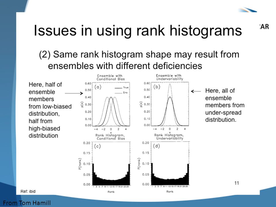
From Tom Hamill

25
Example of Quantile Regression (QR) Our application Fitting T quantiles using QR conditioned on: 1)Ranked forecast ens 2)ensemble mean 3)ensemble median 4) ensemble stdev 5) Persistence R package: quantreg
 Our application Fitting T quantiles using QR conditioned on: 1)Ranked forecast ens 2)ensemble mean 3)ensemble median 4) ensemble stdev 5) Persistence R package: quantreg")
26
T [K] Time forecastsobserved Regressor set: 1. reforecast ens 2. ens mean 3. ens stdev 4. persistence 5. LR quantile (not shown) Probability/°K Temperature [K] climatological PDF Step I: Determine climatological quantiles Step 2: For each quan, use “forward step-wise cross-validation” to iteratively select best subset Selection requirements: a) QR cost function minimum, b) Satisfy binomial distribution at 95% confidence If requirements not met, retain climatological “prior” 1. 3. 2. 4. Step 3: segregate forecasts into differing ranges of ensemble dispersion and refit models (Step 2) uniquely for each range Time forecasts T [K] I.II.III.II.I. Probability/°K Temperature [K] Forecast PDF prior posterior Final result: “sharper” posterior PDF represented by interpolated quans
![T [K] Time forecastsobserved Regressor set: 1. reforecast ens 2.](http://images.slideplayer.com/24/7327305/slides/slide_26.jpg "ens mean 3. ens stdev 4. persistence 5. LR quantile (not shown) Probability/°K Temperature [K] climatological PDF Step I: Determine climatological quantiles Step 2: For each quan, use forward step-wise cross-validation to iteratively select best subset Selection requirements: a) QR cost function minimum, b) Satisfy binomial distribution at 95% confidence If requirements not met, retain climatological prior Step 3: segregate forecasts into differing ranges of ensemble dispersion and refit models (Step 2) uniquely for each range Time forecasts T [K] I.II.III.II.I. Probability/°K Temperature [K] Forecast PDF prior posterior Final result: sharper posterior PDF represented by interpolated quans.")
27
Rank Probability Score for multi-categorical or continuous variables

28
Scatter-plot and Contingency Table Does the forecast detect correctly temperatures above 18 degrees ? Slide from Barbara Casati Brier Score y = forecasted event occurence o = observed occurrence (0 or 1) i = sample # of total n samples => Note similarity to MSE
 i = sample # of total n samples => Note similarity to MSE.")
29
Other post-processing approaches … 1) Bayesian Model Averaging (BMA) – Raftery et al (1997) 2) Analogue approaches – Hopson and Webster, J. Hydromet (2010) 3) Kalman Filter with analogues – Delle Monache et al (2010) 4) Quantile regression – Hopson and Hacker, MWR (under review) 5) quantile-to-quantile (quantile matching) approach – Hopson and Webster J. Hydromet (2010) … many others
 3) Kalman Filter with analogues – Delle Monache et al (2010) 4) Quantile regression – Hopson and Hacker, MWR (under review) 5) quantile-to-quantile (quantile matching) approach – Hopson and Webster J. Hydromet (2010) … many others.")
30
Quantile Matching : another approach when matched forecasts-observation pairs are not available => useful for climate change studies 2004 Brahmaputra Catchment-averaged Forecasts -black line satellite observations -colored lines ensemble forecasts -Basic structure of catchment rainfall similar for both forecasts and observations -But large relative over-bias in forecasts ECMWF 51-member Ensemble Precipitation Forecasts compared To observations

31
Pmax 25th50th75th100th Pfcst Precipitation Quantile Pmax 25th50th75th100th Padj Quantile Forecast Bias Adjustment -done independently for each forecast grid (bias-correct the whole PDF, not just the median) Model Climatology CDF“Observed” Climatology CDF In practical terms … Precipitation 01m ranked forecasts Precipitation 01m ranked observations Hopson and Webster (2010)
 Model Climatology CDF Observed Climatology CDF In practical terms … Precipitation 01m ranked forecasts Precipitation 01m ranked observations Hopson and Webster (2010)")
32
Brahmaputra Corrected Forecasts Original Forecast Corrected Forecast => Now observed precipitation within the “ensemble bundle” Bias-corrected Precipitation Forecasts

Similar presentations


 Yuejian Zhu (EMC) Tom Workoff (WPC) Kathryn Gilbert (MDL) Mike Charles (CPC) Hank Herr (OHD) Trevor.>")


, 2 Centro de Investigaciones.>")


