1. Basic dynamics  The equations of motion and continuity Scaling Hydrostatic relation Boussinesq approximation  Geostrophic balance in ocean’s interior

2. Newton’s second law in a rotating frame. (Navier-Stokes equation) The Equation of Motion : Acceleration relative to axis fixed to the earth. : Pressure gradient force. : Coriolis force, where : Effective (apparent) gravity. : Friction. molecular kinematic viscosity. g 0 =9.80m/s 2 1sidereal day =86164s 1solar day = 86400s

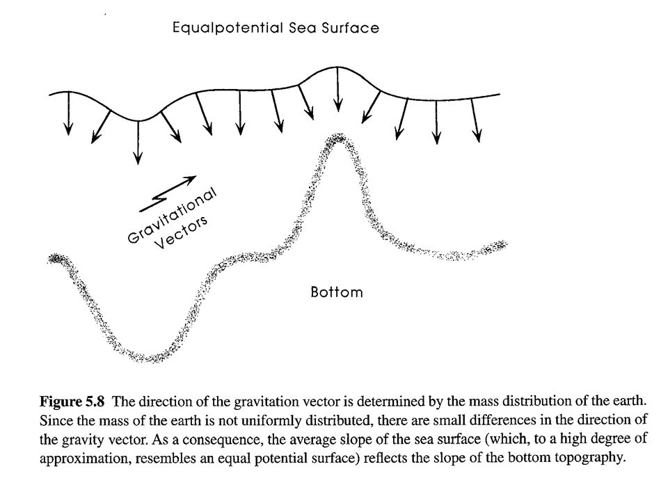
4. Gravity: Equal Potential Surfaces g changes about 5% 9.78m/s 2 at the equator (centrifugal acceleration 0.034m/s 2, radius 22 km longer) 9.83m/s 2 at the poles) equal potential surface normal to the gravitational vector constant potential energy the largest departure of the mean sea surface from the “level” surface is about 2m (slope 10 -5 ) The mean ocean surface is not flat and smooth earth is not homogeneous

7. In Cartesian Coordinates: where

8. Accounting for the turbulence and averaging within T:

9. Given the zonal momentum equation If we assume the turbulent perturbation of density is small i.e., The mean zonal momentum equation is Where F x is the turbulent (eddy) dissipation If the turbulent flow is incompressible, i.e.,

10. Eddy Dissipation A x =A y ~10 2 -10 5 m 2 /s A z ~10 -4 -10 -2 m 2 /s >> Reynolds stress tensor and eddy viscosity: Where the turbulent viscosity coefficients are anisotropic., Then

11. (incompressible) Reynolds stress has no symmetry: A more general definition:    if

12. Continuity Equation Mass conservation law In Cartesian coordinates, we have or For incompressible fluid, If we define and, the equation becomes

13. Scaling of the equation of motion Consider mid-latitude (  ≈45 o ) open ocean away from strong current and below sea surface. The basic scales and constants: L=1000 km = 10 6 m H=10 3 m U= 0.1 m/s T=10 6 s (~ 10 days) 2  sin45 o =2  cos45 o ≈2x7.3x10 -5 x0.71=10 -4 s -1 g≈10 m/s 2  ≈10 3 kg/m 3 A x =A y =10 5 m 2 /s A z =10 -1 m 2 /s Derived scale from the continuity equation W=UH/L=10 -4 m/s  

14. Scaling the vertical component of the equation of motion   Hydrostatic Equation accuracy 1 part in 10 6

15. Boussinesq Approximation Consider a hydrostatic and isentropic fluid  Local scale height   The motion has vertical scale small compared with the scale height

16. Boussinesq approximation Density variations can be neglected for its effect on mass but not on weight (or buoyancy). Assume that where, we have where  Then the equations are where (1) (2) (3) (4) (The term is neglected in (1) for energy consideration.)

17. Geostrophic balance in ocean’s interior

18. Scaling of the horizontal components Zero order (Geostrophic) balance Pressure gradient force = Coriolis force  (accuracy, 1% ~ 1‰)

19. Re-scaling the vertical momentum equation Since the density and pressure perturbation is not negligible in the vertical momentum equation, i.e.,,, and The vertical pressure gradient force becomes

20. Taking into the vertical momentum equation, we have If we scale,and assume then  and (accuracy ~ 1‰)

21. Geopotential Geopotential  is defined as the amount of work done to move a parcel of unit mass through a vertical distance dz against gravity is (unit of  : Joules/kg=m 2 /s 2 ). The geopotential difference between levels z 1 and z 2 (with pressure p 1 and p 2 ) is

22. Dynamic height Given, we have where is standard geopotential distance (function of p only) is geopotential anomaly. In general,  is sometime measured by the unit “dynamic meter” (1dyn m = 10 J/kg). which is also called as “dynamic distance” (D) Note: Though named as a distance, dynamic height (D) is still a measure of energy per unit mass. Units:  ~m 3 /kg, p~Pa, D~ dyn m

23. Geopotential and isobaric surfaces Geopotential surface: constant , perpendicular to gravity, also referred to as “level surface” Isobaric surface: constant p. The pressure gradient force is perpendicular to the isobaric surface. In a “stationary” state (u=v=w=0), isobaric surfaces must be level (parallel to geopotential surfaces). In general, an isobaric surface (dashed line in the figure) is inclined to the level surface (full line). In a “steady” state ( ), the vertical balance of forces is The horizontal component of the pressure gradient force is

25. Geostrophic relation The horizontal balance of force is where tan(i) is the slope of the isobaric surface. tan (i) ≈ 10 -5 (1m/100km) if V 1 =1 m/s at 45 o N (Gulf Stream). In principle, V 1 can be determined by tan(i). In practice, tan(i) is hard to measure because (1) p should be determined with the necessary accuracy (2) the slope of sea surface (of magnitude <10 -5 ) can not be directly measured (probably except for recent altimetry measurements from satellite.) (Sea surface is a isobaric surface but is not usually a level surface.)

26. Calculating geostrophic velocity using hydrographic data The difference between the slopes (i1 and i2) at two levels (z1 and z1) can be determined from vertical profiles of density observations. Level 1: Level 2: Difference: i.e.,  because A 1 C 1 =A 2 C 2 =L and B 1 C 1 -B 2 C 2 =B 1 B 2 -C 1 C 2  because C 1 C 2 =A 1 A 2 Note that z is negative below sea surface.

27. Since and, we have The geostrophic equation becomes