1. Estimation of Statistical Parameters
Estimation theory is a branch of statistics based on measured/empirical data that has a random component.
An estimator attempts to approximate the unknown parameters using the measurements.
In statistics, estimation refers to the process by which one makes inferences about a population, based on information obtained from a sample

2. OUTLINE
Objectives:
Describe the characteristics of the normal distribution in statistical terms
Explain the concept of a confidence interval and how it relates to an estimated parameter

3. Point Estimate vs. Interval Estimate
Statisticians use sample statistics to estimate population parameters.
For example:
sample means are used to estimate population means;
sample proportions, to estimate population proportions.

4. An estimate of a population parameter may be expressed in:
Point Estimate vs. Interval Estimate
An estimate of a population parameter may be expressed in:
Point estimate.
A point estimate of a population parameter is a single value of a statistic.
For example, the sample mean x is a point estimate of the population mean μ.
Similarly, the sample proportion p is a point estimate of the population proportion P.
Interval estimate.
An interval estimate is defined by two numbers, between which a population parameter is said to lie.
For example, a < x < b is an interval estimate of the population mean μ. It indicates that the population mean is greater than a but less than b.

5. the sample statistic + margin of error.
Confidence Intervals
Statisticians use a confidence interval to express the precision and uncertainty associated with a particular sampling method.
A confidence interval consists of three parts.
A confidence level.
A statistic.
A margin of error.
The confidence level describes the uncertainty of a sampling method.
The statistic and the margin of error define an interval estimate that describes the precision of the method.
The interval estimate of a confidence interval is defined by:
the sample statistic + margin of error.
The probability part of a confidence interval is called a confidence level.
The confidence level describes how strongly we believe that a particular sampling method will produce a confidence interval that includes the true population parameter.

6. Standard Error
To compute a confidence interval for a statistic, you need to know the the standard deviation or the standard error of the statistic.
This lesson describes how to find the standard deviation and standard error, and shows how the two measures are related

7. Notation
The following notation is helpful, when we talk about the standard deviation and the standard error.
Population parameter
Sample statistic
N: Number of observations in the population
n: Number of observations in the sample
μ: Population mean
x: Sample estimate of population mean
σ: Population standard deviation
s: Sample estimate of σ

8. Standard Deviation of Sample Estimates
Statisticians use sample statistics to estimate population parameters. Naturally, the value of a statistic may vary from one sample to the next.
The variability of a statistic is measured by its standard deviation.
Statistic
Standard Deviation
Population mean  
𝜎 𝑥 = 𝜎 𝑛
Statistic
Standard Error
Sample mean,  𝑥
𝑆𝐸 𝑥 = 𝑠 𝑛
The equations for the standard error are identical to the equations for the standard deviation, except for one thing - the standard error equations use statistics where the standard deviation equations use parameters. Specifically, the standard error equations use p in place of P, and s in place of σ.

9. Central Limit Theorem
The distribution of sample means (sampling distribution) from a population is approximately normal if the sample size is large, i.e.,
1. The population distribution can be non-normal.
2. Given the population has mean m, then the mean of
the sampling distribution,
3. if the population has variance s2, the standard deviation of the sampling distribution, or the standard error (a measure of the amount of sampling error) is

10. Estimation & Confidence Intervals
Normal distribution:
Gaussian distribution
Symmetric
Not skewed
Unimodal
Described by two parameters:
Probability density function:
μ & σ are parameters
μ = mean
σ = standard deviation
π, e = constants

11. Estimation of Confidence Intervals
Normal distribution: Why do we use it!
Many biological variables follow a normal distribution
The normal distribution is well-understood, mathematically
Punctual estimation
Is a value for estimated theoretical parameter
m (sample mean) is a punctual estimation of μ (population mean)
Is influenced by the fluctuations from sampling
Could be very far away from the real value of the estimated parameter

12. Point Estimations

13. Why Confidence Intervals?
We are not only interested in finding the point estimate for the mean, but also determining how accurate the point estimate is. The Central Limit Theorem plays a key role here. We assume that the sample standard deviation is close to the population standard deviation (which will almost always be true for large samples). Then the Central Limit Theorem tells us that the standard deviation of the sampling distribution is
We will be interested in finding an interval around x such that there is a large probability that the actual mean falls inside of this interval. 
This interval is called a confidence interval and the large probability is called the confidence level.

14. Definitions
A range around the sample estimate in which the population estimate is expected to fall with a specified degree of confidence, usually 95% of the time at a significance level of 5%.
P[lower critical value < estimator < higher critical value] = 1-α
α = significance level
The range defined by the critical values will contains the population estimator with a probability of 1-α
It is applied when variables are normal distributed!

16. Confidence Intervals Definition 1:
95% Confidence Interval for m:
Definition 1:
You can be 95% sure that the true mean (μ) will fall within the upper and lower bounds.
Definition 2:
95% of the intervals constructed using sample means ( x ) will contain the true mean ( μ ).

17. Confidence Intervals It is calculated taking into consideration:
The sample or population size
The type of investigated variable (qualitative OR quantitative)
Formula of calculus comprised two parts:
One estimator of the quality of sample based on which the population estimator was computed (standard error)
Standard error: is a measure of how good our best guess is.
Standard error: the bigger the sample, the smaller the standard error.
Standard error: i always smaller than the standard deviation
Degree of confidence (Zα score)
It is possible to be calculated for any estimator but is most frequent used for mean

18. Confidence Intervals for Means
Standard error of mean is equal to standard deviation divided by square root of number of observations:
If standard deviation is high, the chance of error in estimator is high
If sample size is large, the chance of error in estimator is small.

19. Confidence Intervals for Means
Lower confidence limit is smaller than the mean
Upper confidence limit is higher than the mean
For the 95% confidence intervals: Z5% = 1.96
For the 99% confidence intervals : Z1% = 2.58

20. Confidence Interval for a Mean When the Population Standard Deviation is Unknown
When the population is normal or if the sample size is large, then the sampling distribution will also be normal, but the use of s to replace s is not that accurate.  
The smaller the sample size the worse the approximation will be.  Hence we can expect that some adjustment will be made based on the sample size.  The adjustment we make is that we do not use the normal curve for this approximation.
Instead, we use the Student t distribution that is based on the sample size.  We proceed as before, but we change the table that we use.  This distribution looks like the normal distribution, but as the sample size decreases it spreads out.  For large n it nearly matches the normal curve.  We say that the distribution has n - 1 degrees of freedom.

21. Confidence Intervals 90% CI : x ± 1.65 ( 𝒔 𝒏 )
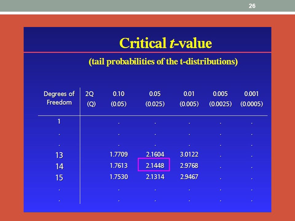
CI for μ if n>120:
90% CI : x ± 1.65 ( 𝒔 𝒏 )
95% CI : x ± 1.96 ( 𝒔 𝒏 )
99% CI : x ± 2.58 ( 𝒔 𝒏 )
CI for μ if n<120:
90% CI : x ± t,n-1 ( 𝒔 𝒏 )
95% CI : x ± t,n-1 ( 𝒔 𝒏 )
99% CI : x ± t,n-1 ( 𝒔 𝒏 )
where t,n-1 distribution is read from table "t" at the  and n-1 degrees of freedom
The EXCEL function T.INV.2T ((probability grade_libertate)

22. GL
0,05
0,01
0,001 2
4,3027
9,925
31,599 46
2,0129
2,687
3,515 89
1,987
2,632
3,403 3
3,1824
5,841
12,924 47
2,0117
2,6846
3,5099 90
3,402 4
2,7764
4,604
8,6103 48
2,0106
2,6822
3,5051 91
1,986
2,631
3,401 5
2,5706
4,032
6,8688 49
2,0096
2,68
3,5004 92
2,63
3,399 6
2,4469
3,707
5,9588 50
2,0086
2,6778
3,496 93
3,398 7
2,3646
3,5
5,4079 51
2,0076
2,6757
3,4918 94
2,629
3,397 8
2,306
3,355
5,0413 52
2,0066
2,6737
3,4877 95
1,985
3,396 9
2,2622
3,25
4,7809 53
2,0057
2,6718
3,4838 96
2,628
3,395 10
2,2281
3,169
4,5869 54
2,0049
2,67
3,48 97
3,394 11
2,201
3,106
4,437 55
2,004
2,6682
3,4764 98
2,627
3,393 12
2,1788
3,055
4,3178 56
2,0032
2,6665
3,4729 99
1,984
2,626
3,392 13
2,1604
3,012
4,2208 57
2,0025
2,6649
3,4696
100
3,391 14
2,1448
2,977
4,1405 58
2,0017
2,6633
3,4663
101
2,625
3,39 15
2,1314
2,947
4,0728 59
2,001
2,6618
3,4632
102
3,389 16
2,1199
2,921
4,015 60
2,0003
2,6603
3,4602
103
1,983
2,624
3,388 17
2,1098
2,898
3,9651 61
1,9996
2,6589
3,4573
104
3,387 18
2,1009
2,878
3,9216 62
1,999
2,6575
3,4545
105
3,386 19
2,093
2,861
3,8834 63
1,9983
2,6561
3,4518
106
2,623
3,385 20
2,086
2,845
3,8495 64
1,9977
2,6549
3,4491
107
1,982
3,384 21
2,0796
2,831
3,8193 65
1,9971
2,6536
3,4466
108
2,622
3,383 22
2,0739
2,819
3,7921 66
1,9966
2,6524
3,4441
109
3,382 23
2,0687
2,807
3,7676 67
1,996
2,6512
3,4417
110
2,621
3,381 24
2,0639
2,797
3,7454 68
1,9955
2,6501
3,4394 25
2,0595
2,787
3,7251 69
1,9949
2,649
3,4372 26
2,0555
2,779
3,7066 70
1,9944
2,6479
3,435 27
2,0518
2,771
3,6896 71
1,9939
2,6469
3,4329 28
2,0484
2,763
3,6739 72
1,9935
2,6459
3,4308 29
2,0452
2,756
3,6594 73
1,993
2,6449
3,4289 30
2,0423
2,75
3,646 74
1,9925
2,6439
3,4269 31
2,0395
2,744
3,6335 75
1,9921
2,643
3,425 32
2,0369
2,739
3,6218 76
1,9917
2,6421
3,4232 33
2,0345
2,733
3,6109 77
1,9913
2,6412
3,4214
111
3,38 34
2,0322
2,728
3,6007 78
1,9908
2,6403
3,4197
112
1,981
2,62 35
2,0301
2,724
3,5911 79
1,9905
2,6395
3,418
113
3,379 36
2,0281
2,72
3,5821 80
1,9901
2,6387
3,4163
114
3,378 37
2,0262
2,715
3,5737 81
1,9897
2,6379
3,4147
115
2,619
3,377 38
2,0244
2,712
3,5657 82
1,989
2,637
3,413
116
3,376 39
2,0227
2,708
3,5581 83
2,636
3,412
117
1,98 40
2,0211
2,705
3,551 84
3,41
118
2,618
3,375 41
2,0195
2,701
3,5442 85
1,988
2,635
3,409
119
3,374 43
2,0167
2,6951
3,5316 86
2,634
3,407
120
2,617 44
2,0154
2,6923
3,5258 87
3,406
>120
1,96
2,576
3,291 45
2,0141
2,6896
3,5203 88
2,633
3,405
Table t

23. Confidence Intervals for Means
The mean of blood sugar concentration of a sample of 121 patients is equal to 105 and the variance is equal to 36.
Which is the confidence levels of blood sugar concentration of the population from which the sample was extracted?
Use a significance level of 5% (Z = 1.96). It is considered that the blood sugar concentration is normal distributed.
n = 121
s2 = 36
s = 6
m = 105
[ ; ]
[103.93; ]
[104;106]

24. Comparing Means by using Confidence Levels
200
100
TAS (mmHg)
Treatament A
Treatament B
Treatament C 𝑥 CI

25. Problem:
A fellow wanted to determine the average serum creatinine level among healthy elderly adult male subjects from Timisoara city. From the literature she could not find any information on on μ or s of serum creatinine among local healthy elderly males. She measured 15 health elderly male volunteers from Timisoara city and the sample mean sCr is 0.94 mg/dL with a sample standard deviation of 0.15 mg/dL. What should be the 95% CI for μ ?

27. Confidence Intervals
Solution:

28. Example
Suppose a student measuring the boiling temperature of a certain liquid observes the readings (in degrees Celsius) 102.5, 101.7, 103.1, 100.9, 100.5, and on 6 different samples of the liquid.
He calculates the sample mean to be
If he knows that the standard deviation for this procedure is 1.2 degrees, what is the confidence interval for the population mean at a 95% confidence level?
In other words, the student wishes to estimate the true mean boiling temperature of the liquid using the results of his measurements. If the measurements follow a normal distribution, then the sample mean will have the distribution N(,/n). Since the sample size is 6, the standard deviation of the sample mean is equal to 1.2/sqrt(6) = 0.49.

29. Remember! High value of standard error Small sample sizes
Correct estimation of a statistical parameter is done with confidence intervals (CI).
Confidence intervals depend by the sample, size and standard error.
The confidence intervals is larger for:
High value of standard error
Small sample sizes