1. F OUNDATIONS OF S TATISTICAL I NFERENCE

2. D EFINITIONS Statistical inference is the process of reaching conclusions about characteristics of an entire population using data from a subset, or sample, of that population. Simple random sampling is a sampling method which ensures that every combination of n members of the population has an equal chance of being selected.

3. Statistical Inference The process of making guesses about the truth about a population parameter from a sample statistic. Sample (observation) Make guesses about the whole population Truth (not observable) Population parameters Sample statistics *hat notation ^ is often used to indicate “estimate”

4. A sampling distribution is the distribution of sample statistics computed on the set of all possible random samples of size n that could be drawn from a population. Most experiments are one-shot deals. So, how do we know if an observed effect from a single experiment is real or is just an artifact of sampling variability (chance variation)? Probability distributions important here. Because they form the basis of describing the distribution of a sample statistic. Sampling Distributions

5. Statistical Inference is based on Sampling Variability Sample Statistic – we summarize a sample into one number; e.g., could be a mean, a difference in means or proportions, an odds ratio, or a correlation or regression coefficient – E.g.: Average support for gun control among women and men. – E.g.: Proportion of women and men who supported the war in Iraq. Sampling Variability – If we could repeat an experiment many, many times on different samples with the same number of subjects, the resultant sample statistic would not always be the same (because of chance!). Standard Error – a measure of the sampling variability. It is the standard deviation of the sampling distribution.

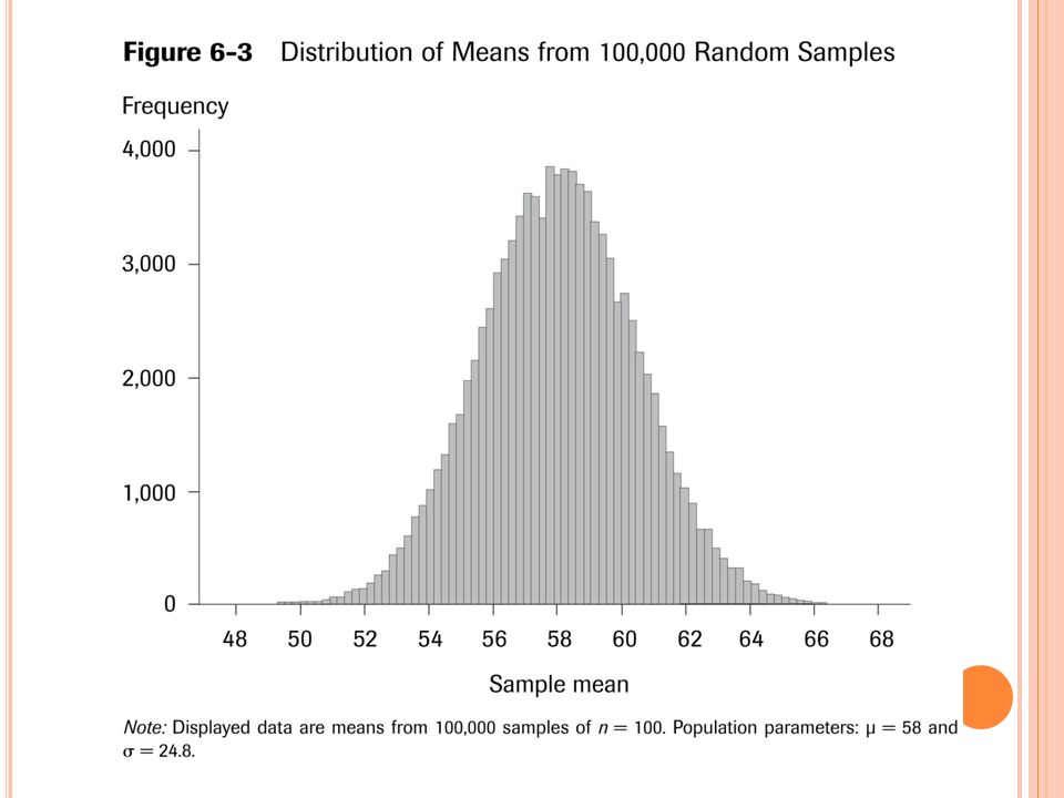
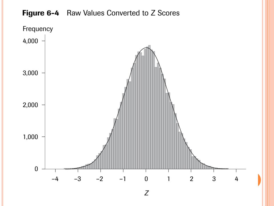
6. For large enough sample sizes, the shape of the sampling distribution will be approximately normal. The sampling distribution is centered on , the mean of the population. The standard deviation of the sampling distribution can be computed as the population standard deviation divided by the square root of the sample size.

7. Examples of Sample Statistics: Single population mean μ (known population standard deviation  ) Single population mean μ (unknown population standard deviation  ) Single population proportion p Difference in means μ 1,μ 2 (t-test) Difference in proportions p 1,p 2 (Z-test) Odds ratio/risk ratio Correlation coefficient Regression coefficient …

8. The Central Limit Theorem: If all possible random samples, each of size n, are taken from any population with a mean  and a standard deviation , the sampling distribution of the sample means (averages) will: 1. Have mean: 2. Have standard deviation (also called standard error for sampling distribution): 3. Be approximately normally distributed regardless of the shape of the parent population (normality improves with larger n).

9. Symbol Check The mean of the sample means. The standard deviation of the sample means. Also called “the standard error of the mean.”

10. I NTUITIVE T REATMENT OF S AMPLING D ISTRIBUTION Suppose we have a population of size 100. We then draw a sample of 100 people from the population of 100. We then compute the mean. How confident could we be about the computed sample statistic? How much sampling error would there be? Suppose we have a population of size 100. We then draw every sample of size 99 from this population. We compute means for all of these samples. How many different samples could we draw? C 99 100 =100? How much sampling error would there be in the computed means? Suppose we have a population of size 100. We then draw a sample of 50 people from the population of 100. We then compute the means on each sample. How many different samples could we draw? C 50 100 =1.089X10 29. How much sampling error would there be in the computed means? The principle is that the larger the sample size, relative to the population we are drawing from, the lower the sampling error. The smaller the sample size, relative to the population we are drawing from, the larger the sampling error.

13. Null Region Alternative Region

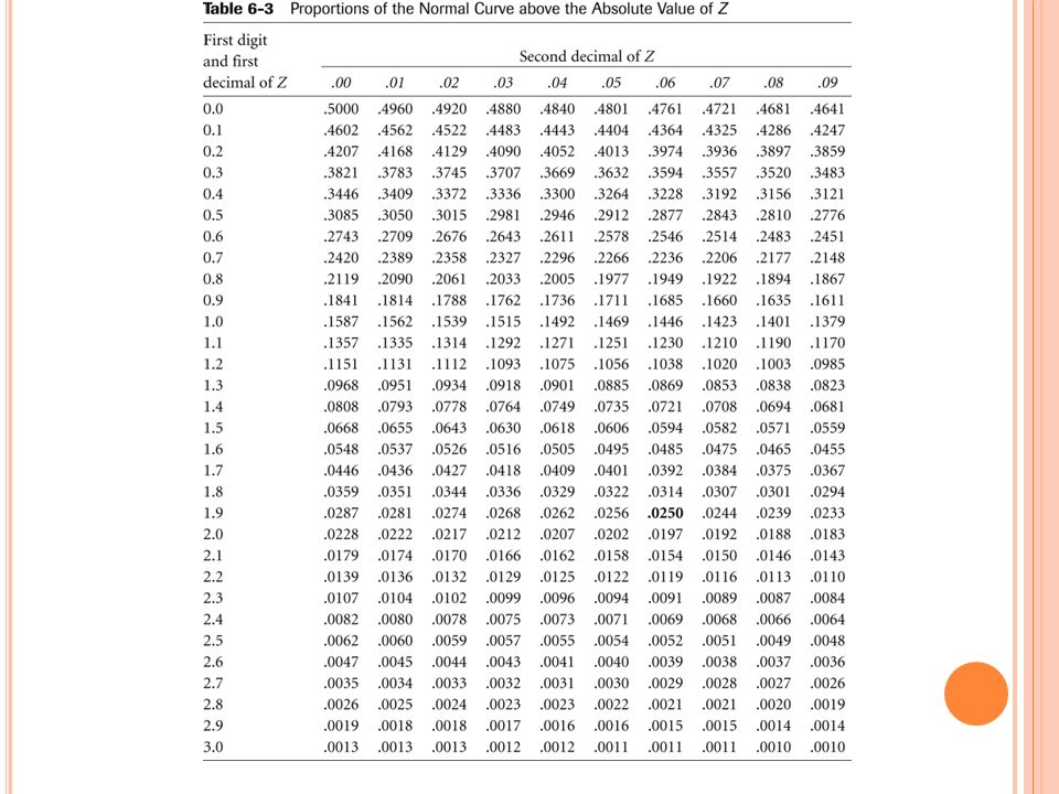
15. H YPOTHESIS T ESTING USING THE N ORMAL (Z) DISTRIBUTION Calculate the estimated statistic from the sample. Record the sample standard deviation  and N. Then calculate the standard error of the sampling distribution from the preceding. Then calculate Z Compare the calculated value for Z to the table of Z statistics.

16. E XAMPLE :. Suppose we draw a sample with mean, variance, and N as follows: How confident could we be that the mean was not actually 10 (the a null hypthesis). We might then ask how many standard deviations (Z units) away 12.5 is from 10. We can then calculate a p value from the Z-statistic. Using the preceding table, there is only a.0016 chance that with a sample of size 50 and variance 36 we could have drawn a sample with mean 12.5 when the actual population mean was 10.

17. E XAMPLE : With the NES92, we draw a sample of 1500 respondents. On the variable, liking for Clinton we find a mean of 4.1 with a variance of 1.6. What is the probability that the real liking for Clinton in the population is only 3, rather than the calculated 4.1? Using the earlier table, the probability is less than 0.001 that the real liking for Clinton is 3.0. What factors determine this probability? 1) The magnitude of the hypothesized difference(the numerator) 2) The variance of the sample (1.6) 3) The N of the sample (1500) Note that we can also think of these three quantities as distances in standard deviation units on the sampling distribution. See slide 13 again.

18. T HE C ONFIDENCE I NTERVAL A PPROACH Let UCL and LCL refer respectively to upper and lower confidence limits. Let μ be the estimated parameter. Let Z be the Z-statistic associated with the desired p-value. Let σ e be the standard error. Then, calculate the confidence limits as follows.

19. E XAMPLE : Construct a 99 percent confidence interval around the point estimate 12.5 from the preceding example with the given information. The interval does not contain zero. Therefore, we can be at least 99 percent confident the estimated mean is not zero. It also does not contain 10, so we can be at least 99 percent confident that the true estimate is not 10.

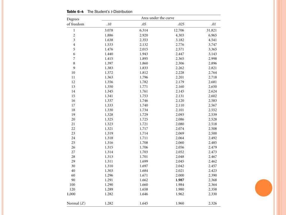
20. U SING THE T - DISTRIBUTION In actuality, we seldom know the population variance or standard deviation. Under these circumstances we use the t distribution, rather than the Z (normal distribution) for our tests of significance. Unlike the Z distribution of which there is only one, there are many t distributions. One for each possible degree of freedom for the test. (Degrees of freedom refer to N minus the number of parameters estimated.) Note, however that as N becomes large, say 100, the t distribution equals the z distribution. The t-distribution is used in precisely the same way as the Z in conducting the preceding tests. Simply substitute in the numbers for the t-distribution where you have the numbers for the Z distribution. The t-distribution takes into account that we do not have full information about the population variability. With small N, the t- distribution is somewhat more conservative than the Z. It gives the same answer if N is larger than about 1,000. It is also quite close when N is larger than about 100. See the next table.

22. T HE P- VALUE The p-value is the probability that we would have observed our sample statistic (or something more unexpected) just by chance if the null hypothesis (null value) is true. For example, we might estimate as above 12.5, but posit a null value of 10. Small p-values mean the null value is unlikely given our data.