Download presentation
Presentation is loading. Please wait.

1
13 PART 5 Perfect Competition
PRICES, PROFITS, AND INDUSTRY PERFORMANCE 13 Perfect Competition CHAPTER

2
C H A P T E R C H E C K L I S T When you have completed your study of this chapter, you will be able to Explain a perfectly competitive firm’s profit- maximizing choices and derive its supply curve. 1 Explain how output, price, and profit are determined in the short run. 2 Explain how output, price, and profit are determined in the long run. 3

3
MARKET TYPES The four market types are Perfect competition Monopoly
Monopolistic competition Oligopoly Launch your lecture by drawing a spectrum of market types noting the four market structures to be studied in this and the next chapters. Let your students know that you will be comparing how a firm in each of these market structures chooses its equilibrium price and equilibrium quantity. Putting this diagram on the board provides a good perspective for the following chapters.

4
Perfect Competition MARKET TYPES Perfect competition exists when
Many firms sell an identical product to many buyers. There are no restrictions on entry into (or exit from) the market. Established firms have no advantage over new firms. Sellers and buyers are well informed about prices.
 the market. Established firms have no advantage over new firms. Sellers and buyers are well informed about prices.")
5
Other Market Types MARKET TYPES
Monopoly is a market for a good or service that has no close substitutes and in which there is one supplier that is protected from competition by a barrier preventing the entry of new firms. Monopolistic competition is a market in which a large number of firms compete by making similar but slightly different products. Oligopoly is a market in which a small number of firms compete.

6
13.1 FIRM’S PROFIT-MAXIMIZING CHOICES
Price Taker A price taker is a firm that cannot influence the price of the good or service that it produces. The firm in perfect competition is a price taker. Once you discuss the characteristics that define perfect competition (many firms selling an identical product to many buyers, no restrictions on entry, established firms have no cost advantage over new firms, and sellers and buyers are well informed about prices) it is natural to give examples of perfectly competitive markets. The examples that always spring to mind are agricultural in nature. Often students, particularly those in urban areas, wonder why they will spend so much of their time studying agriculture. You need to combat the natural view that the model of perfect competition applies only to farms. There are two, complementary paths you can take: First, tell your students that although agriculture certainly meets all the requirements of perfect competition, a lot of other industries come close. If you have a mall near by, you can assign your students to walk through the mall and take note of the different types of businesses and list those that they think are closest to perfect competition. Businesses such as shoe stores, jewelry, toy stores, book stores, hair salons, and so forth are all commonly found in malls and are all relatively close to being in perfectly competitive markets. For instance, you can point out to the students that one jewelry store’s products aren’t identical to those of any other jewelry store, but they are very close substitutes. So, although the jewelry market does not exactly meet the definition of a perfectly competitive market, nonetheless it is likely close enough so that if we want to understand the forces that affect firms within this industry, perfect competition is a reasonable starting point. [Continued on the next slide]
 it is natural to give examples of perfectly competitive markets. The examples that always spring to mind are agricultural in nature. Often students, particularly those in urban areas, wonder why they will spend so much of their time studying agriculture. You need to combat the natural view that the model of perfect competition applies only to farms. There are two, complementary paths you can take: First, tell your students that although agriculture certainly meets all the requirements of perfect competition, a lot of other industries come close. If you have a mall near by, you can assign your students to walk through the mall and take note of the different types of businesses and list those that they think are closest to perfect competition. Businesses such as shoe stores, jewelry, toy stores, book stores, hair salons, and so forth are all commonly found in malls and are all relatively close to being in perfectly competitive markets. For instance, you can point out to the students that one jewelry store’s products aren’t identical to those of any other jewelry store, but they are very close substitutes. So, although the jewelry market does not exactly meet the definition of a perfectly competitive market, nonetheless it is likely close enough so that if we want to understand the forces that affect firms within this industry, perfect competition is a reasonable starting point. [Continued on the next slide]")
7
13.1 FIRM’S PROFIT-MAXIMIZING CHOICES
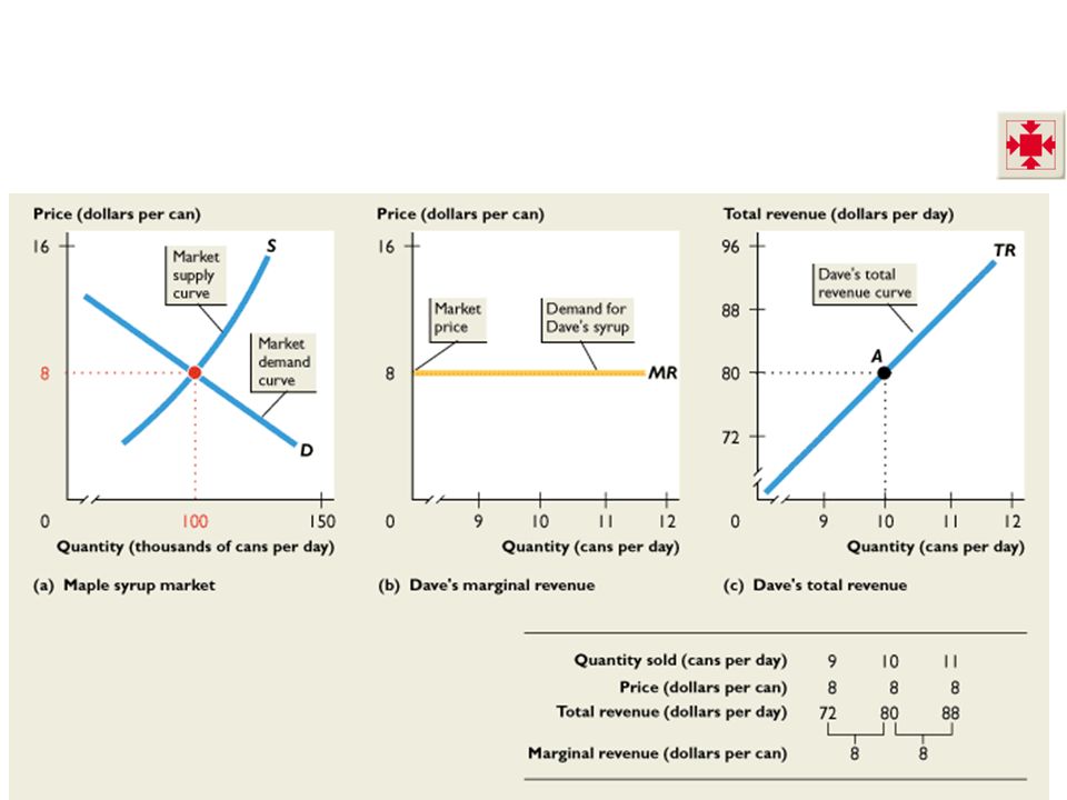
Revenue Concepts In perfect competition, market demand and market supply determine price. A firm’s total revenue equals the market price multiplied by the quantity sold. A firm’s marginal revenue is the change in total revenue that results from a one-unit increase in the quantity sold. Figure 13.1 on the next slide illustrates the revenue concepts. Second, you can use a physical analogy. Ask your students how many of them have taken physics and encountered the assumption of a perfect vacuum. A perfect vacuum cannot exist and our world is not close to being a perfect vacuum. Yet physicists often use the model of a perfect vacuum to understand our physical world. For example, to predict how long it will take a 50 pound steel ball to hit the ground if it is dropped from the top of the Empire State Building, you will be very close to the actual time if you assume a perfect vacuum and use the formula that applies in that case. Friction from the atmosphere is obviously not zero, but assuming it to be zero is not very misleading. In contrast, if you want to predict how long it will take a feather to make the same trip, you need a fancier model! Economists use the model of “perfect competition” in a similar way to understand our economic world. Emphasize to students that although no real world industry meets the full definition of perfect competition, the behavior of firms in many real world industries and the resulting dynamics of their market prices and quantities can be predicted to a high degree of accuracy by using the model of perfect competition.

8
13.1 FIRM’S PROFIT-MAXIMIZING CHOICES
Show what is meant by the term “price taker” by drawing the market supply and market demand curves and the resulting equilibrium price on the left side of the board and then draw the firm’s demand and marginal revenue curves on a separate graph on the right side of the board. Draw a dotted line across from the market graph to the firm graph. Really emphasize the fact that the market demand differs from the firm’s demand because the firm is such a small part of the market. Students consistently confuse the difference between the market demand and the firm’s demand, so the more time you spend clearly explaining this distinction, the better. Part (a) shows the market for maple syrup. The market price is $8 a can.
 shows the market for maple syrup. The market price is $8 a can.")
9
13.1 FIRM’S PROFIT-MAXIMIZING CHOICES
In part (b), the market price determines the demand curve for the Dave’s syrup, which is also his marginal revenue curve.
, the market price determines the demand curve for the Dave’s syrup, which is also his marginal revenue curve.")
10
13.1 FIRM’S PROFIT-MAXIMIZING CHOICES
In part (c), if Dave sells 10 cans of syrup a day, his total revenue is $80 a day at point A.
, if Dave sells 10 cans of syrup a day, his total revenue is $80 a day at point A.")
11
13.1 FIRM’S PROFIT-MAXIMIZING CHOICES
Dave’s total revenue curve is TR. The table shows the calculations of TR and MR.

13
13.1 FIRM’S PROFIT-MAXIMIZING CHOICES
Profit-Maximizing Output As output increases, total revenue increases. But total cost also increases. Because of decreasing marginal returns, total cost eventually increases faster than total revenue. There is one output level that maximizes economic profit, and a perfectly competitive firm chooses this output level.

14
13.1 FIRM’S PROFIT-MAXIMIZING CHOICES
One way to find the profit-maximizing output is to use a firm’s total revenue and total cost curves. Profit is maximized at the output level at which total revenue exceeds total cost by the largest amount. Figure 13.2 on the next slide illustrates this approach.

15
13.1 FIRM’S PROFIT-MAXIMIZING CHOICES
Total revenue increases as the quantity increases —shown by the TR curve. Total cost increases as the quantity increases—shown by the TC curve. As the quantity increases, economic profit (TR – TC) increases, reaches a maximum, and then decreases.
 increases, reaches a maximum, and then decreases.")
16
13.1 FIRM’S PROFIT-MAXIMIZING CHOICES
At low output levels, the firm incurs an economic loss. When total revenue exceeds total cost, the firm earns an economic profit. Profit is maximized when the gap between total revenue and total cost is the largest, at 10 cans per day.

18
13.1 FIRM’S PROFIT-MAXIMIZING CHOICES
Marginal Analysis and the Supply Decision Marginal analysis compares marginal revenue, MR, with marginal cost, MC. As output increases, marginal revenue remains constant but marginal cost increases. If marginal revenue exceeds marginal cost (if MR > MC), the extra revenue from selling one more unit exceeds the extra cost incurred to produce it. Economic profit increases if output increases.
, the extra revenue from selling one more unit exceeds the extra cost incurred to produce it. Economic profit increases if output increases.")
19
13.1 FIRM’S PROFIT-MAXIMIZING CHOICES
If marginal revenue is less than marginal cost (if MR < MC), the extra revenue from selling one more unit is less than the extra cost incurred to produce it. Economic profit increases if output decreases. If marginal revenue equals marginal cost (if MR = MC), the extra revenue from selling one more unit is equal to the extra cost incurred to produce it. Economic profit decreases if output increases or decreases, so economic profit is maximized.
, the extra revenue from selling one more unit is less than the extra cost incurred to produce it. Economic profit increases if output decreases. If marginal revenue equals marginal cost (if MR = MC), the extra revenue from selling one more unit is equal to the extra cost incurred to produce it. Economic profit decreases if output increases or decreases, so economic profit is maximized.")
20
13.1 FIRM’S PROFIT-MAXIMIZING CHOICES
Figure 13.3 shows the profit-maximizing output. Marginal revenue is a constant $8 per can.

21
13.1 FIRM’S PROFIT-MAXIMIZING CHOICES
Figure 13.3 shows the profit-maximizing output. Marginal cost decreases at low outputs but then increases.

22
13.1 FIRM’S PROFIT-MAXIMIZING CHOICES
Figure 13.3 shows the profit-maximizing output. Profit is maximized when marginal revenue equals marginal cost at 10 cans a day.

23
13.1 FIRM’S PROFIT-MAXIMIZING CHOICES
Figure 13.3 shows the profit-maximizing output. If output increases from 9 to 10 cans a day, marginal cost is $7, which is less than the marginal revenue of $8 and profit increases.

24
13.1 FIRM’S PROFIT-MAXIMIZING CHOICES
Figure 13.3 shows the profit-maximizing output. Every term you probably have students who ask, “Do firms really choose the output that maximizes profit?” To answer this question, perhaps before it is asked, it is useful to explain to your students that many big firms routinely make tables using spreadsheets of total revenue, total cost, and economic profit. But most firms, and certainly most small firms, don’t make such calculations. Nonetheless, they do make their decisions at the margin. They can figure out how much it will cost to hire one more worker and how much output that worker will produce. So they can figure out their marginal cost—wage rate divided by marginal product. They can compare that number with the price. They are choosing at the margin as our model of perfect competition assumes. If output increases from 10 to 11 cans a day, marginal cost is $9, which exceeds the marginal revenue of $8 and profit decreases.

25
You always will have students asking why the firm bothers to produce the precise unit of output for which MR = MC. Indeed, it is simply amazing how many students “worry” about this one particular unit of output! Try the following: Draw the conventional upward-sloping MC curve and horizontal MR curve. Make sure to draw these so that the firm will produce a good deal of output. Then, starting at 0, move a bit to the right along the horizontal axis and stop at a point. Tell the students that this point measures 1 unit of output and ask them if this unit should be produced. The answer ought to be yes, because you have arranged matters so MR > MC. Pick some numbers—say, MR = $10 and MC = $1. Ask your students what the profit is for this unit and what the firm’s total profit is if it produces only 1 unit. The answers are $9 and $9. Below the x-axis, label two rows, one called “profit on the unit” and the other “total profit.” Put $9 and $9 in each space under your 1 unit of output. Then move your finger a bit more along the horizontal axis until you come to where you will define the second unit of output. Ask your students if this second unit should be produced. Again, the answer ought to be yes, because you have arranged matters so MR > MC. Pick another number for MC, say $2. Ask your students what the profit is on this unit and what the firm’s total profit is if it produces 2 units. The answers are $8 and $17. Stress that the total profit is what interests the firm and the total profit equals the sum of the profit from the first unit plus the profit from the second unit. Pick a couple of more units and use numbers until you fell it is safe to generalize that the firm produces a unit of output as long as MR > MC. Then, slide your finger to the right, stopping at closer and closer intervals, asking the class if that particular unit should be produced. Always stress that the firm’s total profit continues to increase, albeit more and more slowly. As you get closer to the magical MR-equal-to-MC point, make your stopping intervals even closer. Finally, when you reach MR = MC, tell the students that although this specific unit yields no profit, to have stopped anywhere before it means that the firm would have lost some profit. So, only by producing where MR = MC will the firm obtain the maximum total profit.

26
13.1 FIRM’S PROFIT-MAXIMIZING CHOICES
Exit and Temporary Shutdown Decisions If a firm is incurring an economic loss that it believes is permanent and sees no prospect of ending, the firm exits the market. If a firm is incurring an economic loss that it believes is temporary, it will remain in the market, and it might produce some output or temporarily shut down. Students are often skeptical that a zero economic profit is an acceptable outcome for an entrepreneur. The key is to reinforce the meaning of normal profit. A rational decision is one that is based on a weighing of the full opportunity cost of each alternative against its full benefits. Opportunity cost includes the benefits from forgone opportunities as well as explicit costs. One of these forgone opportunities for the entrepreneur is pursuing his or her next best activity. The value of this forgone opportunity is normal profit. So, when a firm earns zero economic profit, the entrepreneur earns normal profit and enjoys the same benefits as those available in the next best activity. There is no incentive to change to the next best activity.

27
13.1 FIRM’S PROFIT-MAXIMIZING CHOICES
If the firm shuts down, it incurs an economic loss equal to total fixed cost. If the firm produces some output, it incurs an economic loss equal to total fixed cost plus total variable cost minus total revenue. If total revenue exceeds total variable cost, the firm’s economic loss is less than total fixed cost. So it pays the firm to produce and incur an economic loss. Explaining whether a firm exits, temporarily shuts down, or produces even though it has an economic loss is difficult because the last two topics are tough for the students to understand. Exit is the easiest for them to understand because they have seen firms fail throughout their life. But, temporary shutdown is harder to explain. You can help them with the intuition by pointing out that the rationale for temporary shutdown isn’t confined to perfect competition and that they can see the phenomenon right around the corner. Many restaurants close on Sunday evening and Monday. Many hairdressers close on Sunday and Monday. Why? Your students will easily figure out that total revenue is less than total variable cost and equivalently that price is less than average variable cost. The mechanics of the shutdown analysis will be a lot easier to explain once the students have thought about these real situations with which they are familiar. Next, students often have a hard time understanding why operating at an economic loss can be the best action. I use a concrete story to help them see this point. I use Wally’s Wiener World (WWW) hot dog cart. Wally has four costs: his variable costs for his hot dogs, buns, and mustard and his fixed cost for the interest he pays for the loan he used to buy his cart. (If you choose, you can make up numbers for each of these costs.) When price is greater than average variable cost, P>AVC, Wally can pay for his hot dogs, buns, and mustard, and he covers part of the interest cost for the cart, his fixed cost. I show that by operating, he can earn enough to pay at least part of his fixed cost, so he should stay open. But if P < AVC, Wally can’t even afford to buy the dogs, buns, and mustard, much less pay for the interest on his loan. In this circumstance, Wally is better off by shutting down.
 hot dog cart. Wally has four costs: his variable costs for his hot dogs, buns, and mustard and his fixed cost for the interest he pays for the loan he used to buy his cart. (If you choose, you can make up numbers for each of these costs.) When price is greater than average variable cost, P>AVC, Wally can pay for his hot dogs, buns, and mustard, and he covers part of the interest cost for the cart, his fixed cost. I show that by operating, he can earn enough to pay at least part of his fixed cost, so he should stay open. But if P < AVC, Wally can’t even afford to buy the dogs, buns, and mustard, much less pay for the interest on his loan. In this circumstance, Wally is better off by shutting down.")
28
13.1 FIRM’S PROFIT-MAXIMIZING CHOICES
If total revenue were less than total variable cost, the firm’s economic loss would exceed total fixed cost. So the firm would shut down temporarily. Total fixed cost is the largest economic loss that the firm will incur. The firm’s economic loss equals total fixed cost when price equals average variable cost. So the firm produces if price exceeds average variable cost and shuts down if average variable cost exceeds price.

29
13.1 FIRM’S PROFIT-MAXIMIZING CHOICES
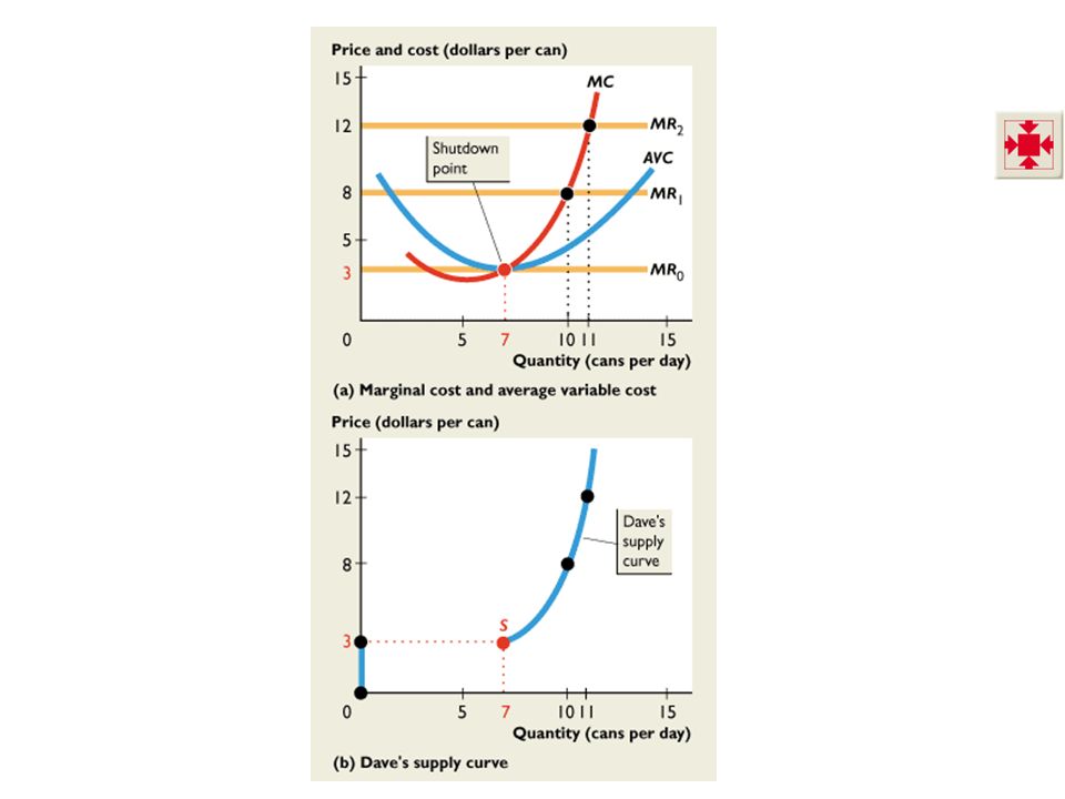
The Firm’s Short-Run Supply Curve A perfectly competitive firm’s short-run supply curve shows how the firm’s profit-maximizing output varies as the price varies, other things remaining the same. The firm’s shutdown point is the output and price at which price equals minimum average variable cost. Figure 13.4 on the next slide illustrates a firm’s supply curve and its relationship to the firm’s cost curves.

30
13.1 FIRM’S PROFIT-MAXIMIZING CHOICES
The firm’s marginal cost curve is MC. Its average variable cost curve is AVC, and its marginal revenue curve is MR0. With a market price (and MR0) of $3 a can, the firm maximizes profit by producing 7 cans a day—at its shutdown point. Point S is one point on the firm’s supply curve.
 of $3 a can, the firm maximizes profit by producing 7 cans a day—at its shutdown point. Point S is one point on the firm’s supply curve.")
31
13.1 FIRM’S PROFIT-MAXIMIZING CHOICES
If the market price rises to $8 a can, the marginal revenue curve shifts upward to MR1. Profit-maximizing output increases to 10 cans per day and the black dot in part (b) is another point of the firm’s supply curve.
 is another point of the firm’s supply curve.")
32
13.1 FIRM’S PROFIT-MAXIMIZING CHOICES
If the price rises to $12 a can, the marginal revenue curve shifts upward to MR2. Profit-maximizing output increases to 11 cans per day and the new black dot in part (b) is another point of the firm’s supply curve.
 is another point of the firm’s supply curve.")
33
13.1 FIRM’S PROFIT-MAXIMIZING CHOICES
The blue curve in part (b) is the firm’s supply curve. At prices below $3 a can, the firm shuts down and output is zero. At prices above $3 a can, the firm produces along its MC curve. The supply curve is the same as the MC curve above the point of minimum AVC.
 is the firm’s supply curve. At prices below $3 a can, the firm shuts down and output is zero. At prices above $3 a can, the firm produces along its MC curve. The supply curve is the same as the MC curve above the point of minimum AVC.")
35
Market Supply in the Short Run
The market supply curve in the short run shows the quantity supplied at each price by a fixed number of firms. The quantity supplied at a given price is the sum of the quantities supplied by all firms at that price.

36
13.2 IN THE SHORT RUN Figure 13.5 shows the market supply curve in a market with 10,000 identical firms. At the shutdown price of $3, each firm produces either 0 or 7 cans a day.

37
13.2 IN THE SHORT RUN At prices below the shutdown price, firms produce no output. At prices above the shutdown price, firms produce along their marginal cost curve.

38
13.2 IN THE SHORT RUN At prices below the shutdown price, the market supply curve runs along the y-axis. At the shutdown price, the market supply curve is perfectly elastic. At prices above the shutdown price, the market supply curve is upward sloping.

40
Short-Run Equilibrium in Good Times
13.2 IN THE SHORT RUN Short-Run Equilibrium in Good Times Market demand and market supply determine the price and quantity bought and sold. Figure 13.6 on the next slide illustrates short-run equilibrium when the firm makes an economic profit.

41
13.2 IN THE SHORT RUN In part (a), with market demand curve D1 and market supply curve S, the price is $8 a can.

42
13.2 IN THE SHORT RUN In part (b), Dave’s marginal revenue is $8 a can, so he produces 10 cans a day, where marginal cost equals marginal revenue.
, Dave’s marginal revenue is $8 a can, so he produces 10 cans a day, where marginal cost equals marginal revenue.")
43
13.2 IN THE SHORT RUN At this quantity, price ($8) exceeds average total cost ($5.10), so Dave makes an economic profit shown by the blue rectangle.
 exceeds average total cost ($5.10), so Dave makes an economic profit shown by the blue rectangle.")
45
Short-Run Equilibrium in Bad Times
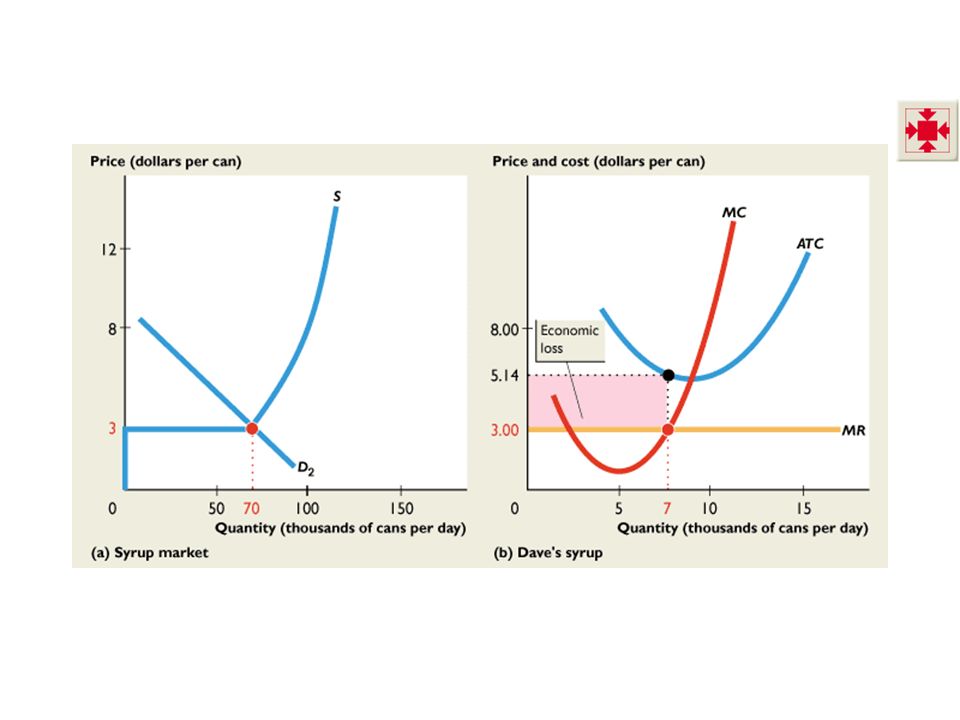
13.2 IN THE SHORT RUN Short-Run Equilibrium in Bad Times In the short-run equilibrium that we’ve just examined, Dave is enjoying an economic profit. But such an outcome is not inevitable. Figure 13.7 on the next slide illustrates short-run equilibrium when the firm incurs an economic loss.

46
13.2 IN THE SHORT RUN In part (a), with market demand curve D2 and market supply curve S, the price is $3 a can.
, with market demand curve D2 and market supply curve S, the price is $3 a can.")
47
13.2 IN THE SHORT RUN In part (b), Dave’s marginal revenue is $3 a can, so he produces 7 cans a day, where marginal cost equals marginal revenue.
, Dave’s marginal revenue is $3 a can, so he produces 7 cans a day, where marginal cost equals marginal revenue.")
48
13.2 IN THE SHORT RUN At this quantity, price ($3) is less than average total cost ($5.14), so Dave incurs an economic loss shown by the red rectangle.
 is less than average total cost ($5.14), so Dave incurs an economic loss shown by the red rectangle.")
50
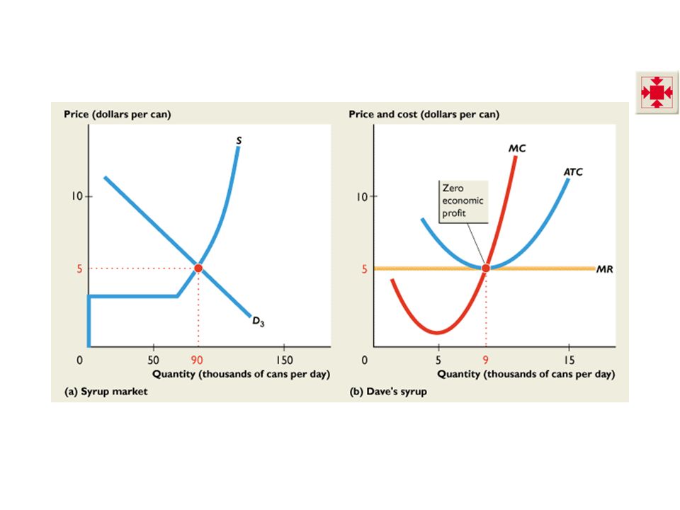
13.3 IN THE LONG RUN Neither good times nor bad times last forever in perfect competition. In the long run, a firm in perfect competition earns normal profit. It earns zero economic profit and incurs no economic loss. Figure 13.8 on the next slide illustrates an equilibrium when the firm earns a normal profit—and zero economic profit.

51
13.3 IN THE LONG RUN In part (a), with market demand curve D3 and market supply curve S, the price is $5 a can.
, with market demand curve D3 and market supply curve S, the price is $5 a can.")
52
13.3 IN THE LONG RUN In part (b), Dave’s marginal revenue is $5 a can, so he produces 9 cans a day, where marginal cost equals marginal revenue.
, Dave’s marginal revenue is $5 a can, so he produces 9 cans a day, where marginal cost equals marginal revenue.")
54
Entry and Exit 13.3 IN THE LONG RUN
In the long run, firms respond to economic profit and economic loss by either entering or exiting a market. New firms enter a market in which the existing firms Entry and exit influence price, the quantity produced, and economic profit.

55
13.3 IN THE LONG RUN The immediate effect of the decision to enter or exit is to shift the market supply curve. If more firms enter a market, supply increases and the market supply curve shifts rightward. If firms exit a market, supply decreases and the market supply curve shifts leftward.

56
13.3 IN THE LONG RUN The Effects of Entry
Economic profit is an incentive for new firms to enter a market, but as they do so, the price falls and the economic profit of each existing firm decreases.

57
13.3 IN THE LONG RUN Figure 13.9 shows the effects of entry.
Starting in long-run equilibrium, 1. If demand increases from D0 to D1, the price rises from $5 to $8 a can. Firms now make economic profit.

58
13.3 IN THE LONG RUN Economic profit brings entry.
2. As firms enter the market, the supply curve shifts rightward, from S0 to S1. The equilibrium price falls from $8 to $5 a can, and the quantity produced increases from 100,000 to 140,000 cans a day.

60
The Effects of Exit 13.3 IN THE LONG RUN
Economic loss is an incentive for firms to exit a market, but as they do so, the price rises and the economic loss of each remaining firm decreases.

61
13.3 IN THE LONG RUN Figure 13.10 shows The effects of exit.
Starting in long-run equilibrium, 1. If demand decreases from D0 to D2, the price falls from $5 to $3 a can. Firms now make economic losses.

62
13.3 IN THE LONG RUN Economic loss brings exit.
2. As firms exit the market, the supply curve shifts leftward, from S0 to S2. The equilibrium price rises from $3 to $5 a can, and the quantity produced decreases from 70,000 to 40,000 cans a day.

64
A Change in Demand 13.3 IN THE LONG RUN
The difference between the initial long-run equilibrium and the final long-run equilibrium is the number of firms in the market. An increase in demand increases the number of firms. Each firm produces the same output in the new long-run equilibrium as initially and earns a normal profit. In the process of moving from the initial equilibrium to the new one, firms make economic profits.

65
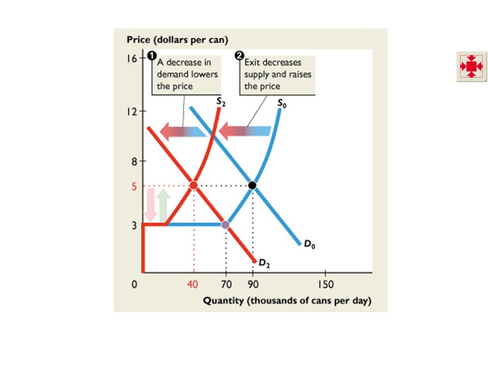
13.3 IN THE LONG RUN A decrease in demand triggers a similar response, except in the opposite direction. The decrease in demand brings a lower price, economic loss, and exit. Exit decreases market supply and eventually raises the price to its original level.

66
Technological Change 13.3 IN THE LONG RUN
New technology allows firms to produce at a lower cost. As a result, as firms adopt a new technology, their cost curves shift downward. Market supply increases, and the market supply curve shifts rightward. With a given demand, the quantity produced increases and the price falls.

67
13.3 IN THE LONG RUN Two forces are at work in a market undergoing technological change. Firms that adopt the new technology make an economic profit. So new-technology firms have an incentive to enter. Firms that stick with the old technology incur economic losses. They either exit the market or switch to the new technology.

68
Is Perfect Competition Efficient?
13.3 IN THE LONG RUN Is Perfect Competition Efficient? The difference between the initial long-run equilibrium and the final long-run equilibrium is the number of firms in the market. An increase in demand increases the number of firms. Each firm produces the same output in the new long-run equilibrium as initially and earns a normal profit. In the process of moving from the initial equilibrium to the new one, firms make economic profits.

69
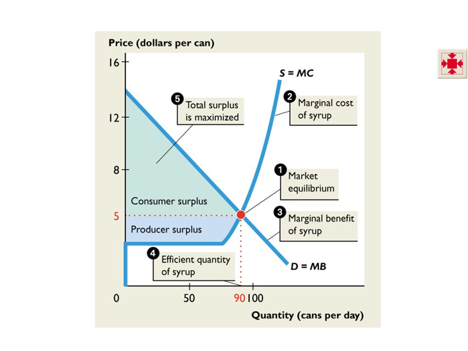
13.3 IN THE LONG RUN 1. Market equilibrium occurs at a price of $5 a can and a quantity of 90 cans a day. 2. Supply curve is also the marginal cost curve. 3. Demand curve is also the marginal benefit curve.

70
13.3 IN THE LONG RUN Because marginal benefit equals marginal cost
4. Efficient quantity is produced. 5. Total surplus (sum of consumer surplus and producer surplus) is maximized.
 is maximized.")
72
Is Perfect Competition Fair?
13.3 IN THE LONG RUN Is Perfect Competition Fair? Perfect competition places no restrictions on anyone’s actions—everyone is free to try to earn an economic profit. The process of competition eliminates economic profit and brings maximum attainable benefit to consumers. Fairness as equality of opportunity and fairness as equality of outcomes are achieved in long-run equilibrium.

73
13.3 IN THE LONG RUN But in the short run, economic profit and economic loss can arise. These unequal outcomes might seem unfair.

74
Perfect Competition in YOUR Life
You don’t run into perfect competition very often. But you do see many markets that are highly competitive. Your entire life is influenced by and benefits from the forces of competition. Adam Smith’s invisible hand might be hidden from view, but it is enormously powerful. Just about every good and service that you consume is available because of the forces of competition. No one organizes all the magic that enables you to consume this vast array of products. But competitive markets and entrepreneurs striving to make the largest possible profit make it happen.

Similar presentations