1. TR-55 Urban Hydrology for Small Watersheds

2. Simplified methods for estimating runoff for small urban/urbanizing watersheds
Ch 1 Intro
Ch 2 Estimating Runoff
Ch 3 Time of Concentration
Ch 4 Peak Runoff Method
Ch 5 Hydrograph Method
Ch 6 Storage Volumes for Detention Basins

3. Appendices A-Hydrologic Soil Groups B-Rainfall Data
C-TR-55 Program (old; outdated)
D-Worksheet Blanks
E-References

4. TR-55 PDF is available at http://www.hydrocad.net/tr-55.htm
Software (WinTR-55) available at

5. Objectives
Know how to estimate peak flows by hand using the TR-55 manual
Know how to obtain soil information

6. TR-55 (General)
Whereas the rational method uses average rainfall intensities the TR-55 method starts with mass rainfall (inches-P) and converts to mass runoff (inches-Q) using a runoff curve number (CN)
CN based on:
Soil type
Plant cover
Amount of impervious areas
Interception
Surface Storage
Similar to the rational method--the higher the CN number the more runoff there will be

7. TR-55 (General) Mass runoff is transformed into peak flow (Ch 4) or
hydrograph (Ch 5) using unit hydrograph theory and routing procedures that depend on runoff travel time through segments of the watershed

8. Rainfall Time Distributions
TR-55 uses a single storm duration of 24 hours to determine runoff and peak volumes
TR-55 includes 4 synthetic regional rainfall time distributions:
Type I-Pacific maritime (wet winters; dry summers)
Type IA-Pacific maritime (wet winters; dry summers-less intense than I)
Type II-Rest of country (most intense)
Type III-Gulf of Mexico/Atlantic Coastal Areas
Rainfall Time Distribution is a mass curve
Most of upstate NY is in Region II

10. Appendix B
24-hr rainfall data for 2,5,10,25,50,and 100 year frequencies

11. Limitations of TR-55
Methods based on open and unconfined flow over land and in channels
Graphical peak method (Ch 4) is limited to a single, homogenous watershed area
For multiple homogenous subwatersheds use the tabular hydrograph method (Ch 5)
Storage-Routing Curves (Ch 6) should not be used if the adjustment for ponding (Ch 4) is used

12. Ch 2 Determine Runoff Curve Number Factors: Hydrologic Soil Group
Cover Type and Treatment
Hydrologic Condition
Antecedent Runoff Condition (ARC)
Impervious areas connected/unconnected to closed drainage system

13. Hydrologic Soil Group A-High infiltration rates
B-Moderate infiltration rates
C-Low infiltration rates
D-High runoff potential

14. Soil Maps
GIS accessible maps are at
Hints:
AOI (polygon; double click to end)
Soil Data Explorer
Soil Properties and Qualities
Soil Qualities and Features
Hydrologic Soil Group
View Rating
Printable Version

15. Cover Type and Treatment
Urban (Table 2-2a)
Cultivated Agricultural Lands (Table 2-2b)
Other Agricultural Lands (Table 2-2c)
Arid/Semiarid Rangelands (Table 2-2d)

16. Hydrologic Condition
Poor
Fair
Good
Description in table 2-2 b/c/d

17. Antecedent Runoff Condition (ARC)
Accounts for variation of CN from storm to storm
Tables use average ARC

18. Impervious/Impervious Areas
Accounts for % of impervious area and how the water flows after it leaves the impervious area
Is it connected to a closed drainage system?
Is it unconnected (flows over another area)?
If unconnected
If impervious <30% then additional infiltration will occur
If impervious >30% then no additional infiltration will occur

19. Table 2-2a Assumptions
Pervious urban areas are equivalent to pasture in good conditions
Impervious areas have a CN of 98
Impervious areas are connected
Impervious %’s as stated in Table
If assumptions not true then modify CN using Figure 2-3 or 2-4

20. Modifying CN using Figure 2-3
If impervious areas are connected but the impervious area percentage is different than Table 2-2a then use Figure 2-3

21. Modifying CN using Figure 2-4
If impervious area < 30% but not connected then use Figure 2-4

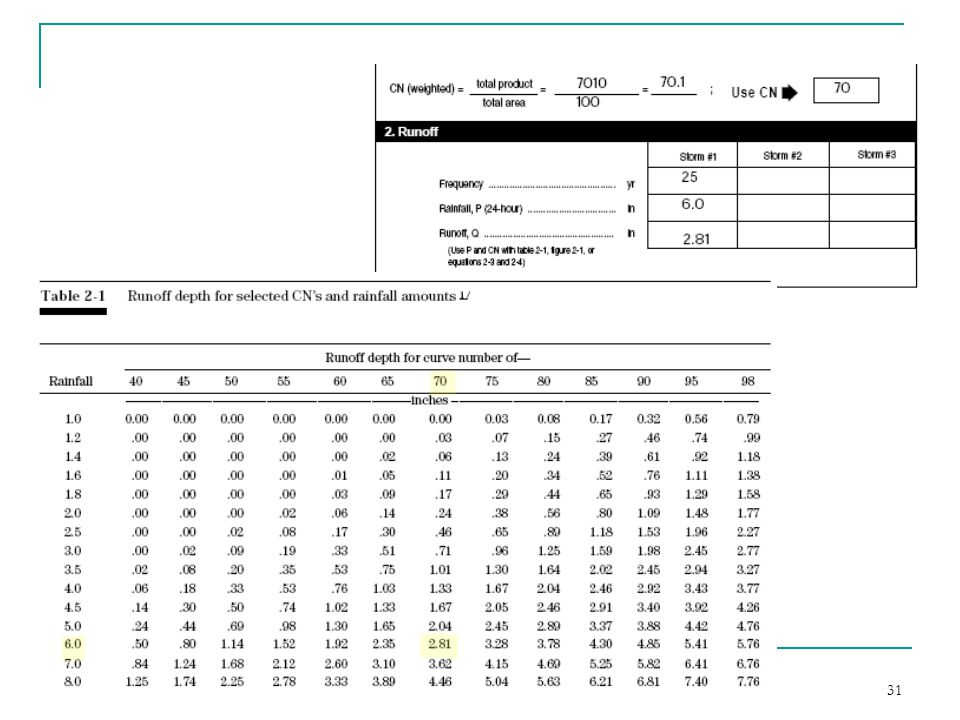
22. Determining Q (runoff in inches)
Find rainfall P (Appendix B)
Find Q from Figure 2-1
Or Table 2-1

23. Determining Q (Table 2-1)

24. Equation S is maximum potential retention of water (inches)
S is a function of the CN number
0.2S is assumed initial abstraction

25. Limitations CN numbers describe average conditions
Runoff equations don’t account for rainfall duration or intensity
Initial abstraction=0.2S (agricultural studies)
Highly urbanized areas—initial abstraction may be less
Significant storage depression---initial abstraction could be more
CN procedure less accurate when runoff < 0.5”
Procedure overlooks large sources of groundwater
Procedure inaccurate when weighted CN<40

26. TR-55 Example

28. Examples Example 2-1 (undeveloped): Example 2-2 (developed):
Impervious/Pervious doesn’t apply
Example 2-2 (developed):
Table assumptions are met
Example 2-3 (developed):
Table assumptions not met (Figure 2-3)
Example 2-4 (developed):
Table assumptions not met (Figure 2-4)

32. Examples Example 2-2: Land is subdivided into lots
Table assumptions are met

35. Examples Example 2-3: Land is subdivided into lots
Table assumptions are not met
Table assumes 25% impervious; actual is 35% impervious
The runoff should be higher since impervious is increased

37. Using Figure 2-3 Pervious CN’s were 61 and 74 Start @ 35%
Open space; good condition; same as first example
35%
Go up to hit CN 61 & 74 curves
Go left to determine new CN=74 & 82

39. Examples Example 2-4: Land is subdivided into lots
Table assumptions are not met
Actual is 25% impervious but 50% is not directly connected and flows over pervious area
Use Figure 2-4
The runoff should be lower since not all the impervious surface is connected (water flows over pervious areas and allows more water to infiltrate)

41. Using Figure 2-4 Pervious CN is 74 50% unconnected
Open space; good condition; same as first example
50% unconnected
the bottom (right 25%
Go up to 50% curve
Go left to pervious CN of 74
Go down to read composite CN of 78

43. Example Comparison Undeveloped Developed (25% impervious connected
Developed (25% impervious but only 50% connected)
Roff=2.81”
Roff=3.28”
Roff=3.48”
Roff=3.19”

44. Time of Concentration & Travel Time Chapter 3
Sheet flow
Shallow Concentrated Flow
Channel Flow
Use Worksheet 3

46. Chapter 4: Graphical Peak Discharge Worksheet 4
Inputs:
Drainage Area
CN (from worksheet 2)
Time of concentration (from worksheet 3)
Appropriate Rainfall Distribution (I/IA/II/III) App B
Rainfall, P (worksheet 2)
Runoff Q (in inches) from worksheet 2
Pond & Swamp Adjustment Factor (Table 4-2)

47. Ch 4 Calculations Find initial abstraction Function of CN #
Find in Table 4-I
Calculate Ia/P

48. Ch 4 Calculations
Determine peak discharge (cubic feet per square mile per inch of runoff) from Exhibit 4-I, 4-IA, 4-II or 4-III by using the Ia/P ratio and the time of concentration

50. Pond & Swamp Adjustment Table 4-2

51. Compute Peak Flow
Peak flow=Unit peak flow * Inches of Runoff * Drainage Area * Pond/swamp Adjustment Factor

53. Limitations Watershed must be hydrologically homogenous
One main stream (not branched)
No reservoir routing
Pond/swamp adjustment factor applied only if not in the time of concentration path
Can’t use if Ia/P values are outside range of
Not accurate if CN<40
Tc between 6 minutes and 10 hours