1. A Parallel Computational Framework for Discontinuous Galerkin Methods Kumar Vemaganti Mechanical Engineering University of Cincinnati

2. Acknowledgements ICES (formerly TICAM), UT Austin Abani Patra, SUNY Buffalo

3. Outline PI-FED in a nutshell Design Considerations Implementation Issues Sample Applications

4. PIFED: Parallel Infrastructure for Finite Element Discretizations Two-dimensional Adaptive FE Conforming and Non-conforming Quadrilaterals and Triangles Parallel: Partitioning through Space Filling Curves Multiple Linear Solvers C++ and some FORTRAN

5. Design Considerations (for a Research Code) Source code available (GPL) Flexible: Multiple Solution Components Extensible: Object Oriented Portable on *NIX: RS6000, IRIX, Linux, Mac OS X Parallel: Distributed Datastructures Adaptive: Dynamic Datastructures

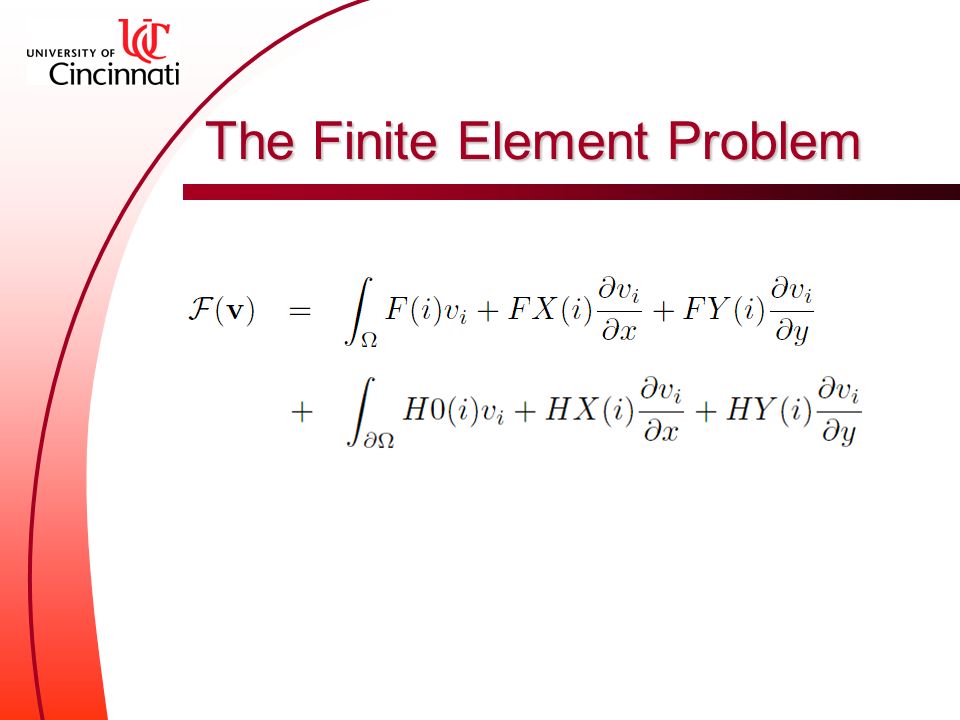
6. The Finite Element Problem

8. Discontinuous Formulations: Additional Terms Additional terms on the LHS: The Finite Element Problem is completely specified if the coefficients A**, B**, F*, H*, J** are specified for each element/edge.

9. Organization PI-FED Library Application (User-supplied) Partitioning DatastructuresCommunications Solvers Domain (Mesh) Coefficients: A**, J**, etc. Control Parameters

10. Non-overlapping Partitioning: Hilbert Space Filling Curves Hilbert SFC: A one-dimensional curve that fills the unit square. SFC Implementation: HSFC2D & HSFC3D (H. Carter Edwards)

11. PIFED: Other Features Solvers: Direct: SPOOLES, SPARSE 1.3 Iterative: PCG & GMRES AZTEC interface in the works Datastructures Hashtables for elements and nodes (gNodes, pNodes) Hash rule based on SFC key Communications MPICH version of MPI Hidden from user

12. Coefficient Function MCOEFF: Element by Element #include "AFE-machine.hh" #include "AFE-3D.hh" subroutine USER_MCOEFF ( xyzloc, xyzglob,. mat, neq, nrhs,. nreal, rval, nint, ival,. unreal, urval, unint, uival,. axx, axy, ayx, ayy,. a0x, a0y, ax0, ay0,. a00, f0, fx, fy )

13. Coefficient Function MCOEFF c-- Fill up the coefficient arrays axx(1,1) = a1111 ayy(1,1) = 0.5d0*a1212 axy(1,2) = a1122 ayx(1,2) = 0.5d0*a1212 axy(2,1) = 0.5d0*a1212 ayx(2,1) = a1122 axx(2,2) = 0.5d0*a1212 ayy(2,2) = a2222 c-- RHS coefficients f0(1,1) = -1.0d0*a1111 f0(2,1) = -1.0d0*a2222

14. /* Dirichlet BCs */ if ( strcmp ( Type, "Displacement" ) == 0 ) { /* LHS terms */ BX0[0+0*(*n_c)] = a1111*unorm[0]; BX0[0+1*(*n_c)] = a1122*unorm[1]; BX0[1+0*(*n_c)] = 0.5*a1212*unorm[1]; BX0[1+1*(*n_c)] = 0.5*a1212*unorm[0]; BY0[0+0*(*n_c)] = 0.5*a1212*unorm[1]; BY0[0+1*(*n_c)] = 0.5*a1212*unorm[0]; BY0[1+0*(*n_c)] = a1122*unorm[0]; BY0[1+1*(*n_c)] = a2222*unorm[1]; Coefficient Function BCOEFF: Boundary Edges

15. Coefficient Function BCOEFF B0X[0+0*(*n_c)] = -1.0*a1111*unorm[0]; B0X[0+1*(*n_c)] = -0.5*a1212*unorm[1]; B0X[1+0*(*n_c)] = -1.0*a1122*unorm[1]; B0X[1+1*(*n_c)] = -0.5*a1212*unorm[0]; B0Y[0+0*(*n_c)] = -0.5*a1212*unorm[1]; B0Y[0+1*(*n_c)] = -1.0*a1122*unorm[0]; B0Y[1+0*(*n_c)] = -0.5*a1212*unorm[0]; B0Y[1+1*(*n_c)] = -1.0*a2222*unorm[1]; /* RHS terms */ hx[0] = u0*unorm[0]*a1111 + u1*unorm[1]*a1122; hx[1] = 0.5*a1212*(u0*unorm[1] + u1*unorm[0]); hy[0] = 0.5*a1212*(u0*unorm[1] + u1*unorm[0]); hy[1] = u0*unorm[0]*a1122 + u1*unorm[1]*a2222; } /* End of Dirichlet BCs */

16. Coefficient Function JCOEFF: Interior Edges c------------------------------------------------- c-- Coefficients for this element c------------------------------------------------- c-- JX0 JX0(1,1) = unorma(1)*a1111 JX0(1,2) = unorma(2)*a1122 JX0(2,1) = 0.5d0*unorma(2)*a1212 JX0(2,2) = 0.5d0*unorma(1)*a1212 c-- JY0 JY0(1,1) = 0.5d0*unorma(2)*a1212 JY0(1,2) = 0.5d0*unorma(1)*a1212 JY0(2,1) = unorma(1)*a1122 JY0(2,2) = unorma(2)*a2222

17. Coefficient Function JCOEFF c------------------------------------------------ c-- Coefficients for neighbor c------------------------------------------------ c-- JX0 JX0_n(1,1) = unorma(1)*n1111 JX0_n(1,2) = unorma(2)*n1122 JX0_n(2,1) = 0.5d0*unorma(2)*n1212 JX0_n(2,2) = 0.5d0*unorma(1)*n1212 c-- JY0 JY0_n(1,1) = 0.5d0*unorma(2)*n1212 JY0_n(1,2) = 0.5d0*unorma(1)*n1212 JY0_n(2,1) = unorma(1)*n1122 JY0_n(2,2) = unorma(2)*n2222

18. Control Parameters // Set the number of post-processing quantities int npost = 5; set_parameter ( NUM_POST_QTY, (void *)&npost ); // Set the number of RHSs int nrhs = 1; set_parameter ( NUM_RHS, (void *)&nrhs ); // Set number of solution components int nc=2; set_parameter ( NUM_COMP, (void *)&nc ); // Set the finite element type to DG int fe_type=NONCONFORMING; set_parameter ( FE_TYPE, (void *)&fe_type );

19. Example: Linear Elasticity Horizontal traction force on right edge Left edge fixed Isotropic Material p-level = 2

20. Results on Initial Mesh Horizontal Displacements Vertical Displacements

21. Results on Initial Mesh von Mises Stress

22. Refined Mesh Horizontal traction force on right edge Left edge fixed Isotropic Material p-level = 2

23. Results on Refined Mesh Horizontal Displacements Vertical Displacements

24. Results on Refined Mesh von Mises Stress

25. Another Example: Topology Optimization Goal: Maximize the stiffness, subject to volume constraints Discrete problem: Determine which elements have material in them, and which ones don' t

26. Extreme Materials

27. Material with Poisson Ratio = -0.95