1. 15.082 and 6.855J The Capacity Scaling Algorithm

2. 2 The Original Costs and Node Potentials 1 2 35 4 4 1 2 2 5 6 7 0 00 00

3. 3 The Original Capacities and Supplies/Demands 1 2 35 4 10 20 25 20 30 23 5-2 -7 -19

4. 4 Set  = 16. This begins the  -scaling phase. 1 2 35 4 10 20 25 20 30 23 5-2 -7 -19 We send flow from nodes with excess   to nodes with deficit  . We ignore arcs with capacity  .

5. 5 Select a supply node and find the shortest paths 1 2 35 4 4 1 2 2 5 6 7 7 0 6 8 8 shortest path distance The shortest path tree is marked in bold and blue.

6. 6 Update the Node Potentials and the Reduced Costs 1 2 35 4 4 1 2 2 5 6 7 0 -7-8 -6 0 0 0 0 6 3 1 To update a node potential, subtract the shortest path distance.

7. 7 Send Flow Along a Shortest Path in G(x, 16) 1 2 3 5 4 1 Send flow from node 1 to node 5. 20 25 20 30 23 5-2 -7 -19 How much flow should be sent? 10

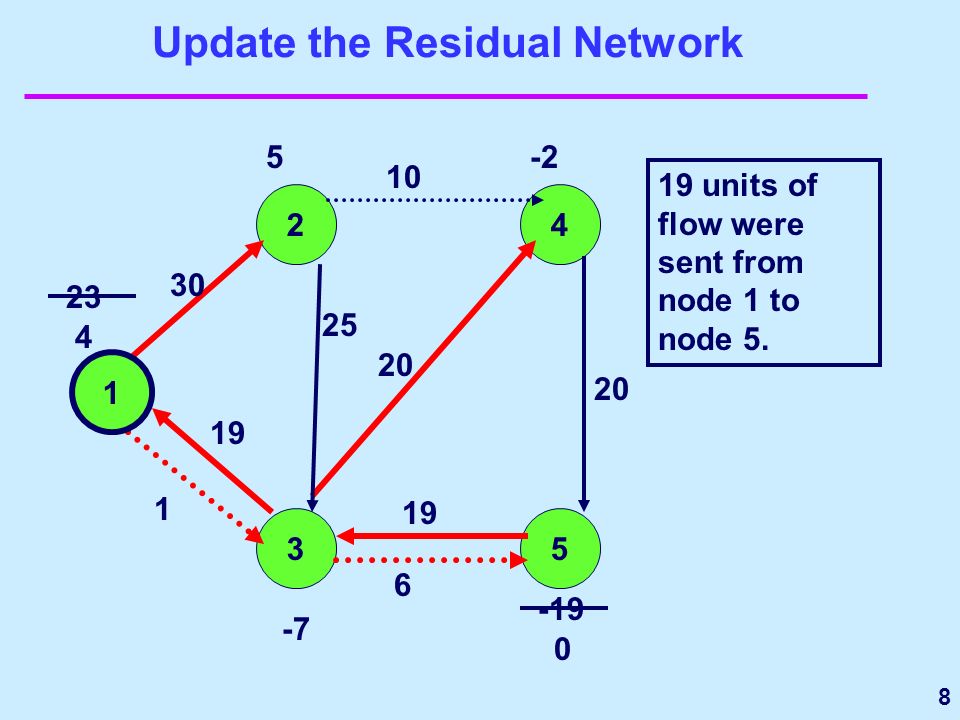
8. 8 Update the Residual Network 1 2 35 4 1 19 units of flow were sent from node 1 to node 5. 20 6 25 1 30 23 5-2 -7 0 10 -19 4 19

9. 9 This ends the 16-scaling phase. 1 2 35 4 1 The  -scaling phase continues when e(i)   for some i. e(j)  -  for some j. There is a path from i to j. 20 6 25 1 30 5-2 -7 0 10 4 19

10. 10 This begins and ends the 8-scaling phase. 1 2 35 4 1 The  -scaling phase continues when e(i)   for some i. e(j)  -  for some j. There is a path from i to j. 20 6 25 1 30 5-2 -7 0 10 4 19

11. 11 This begins 4-scaling phase. 1 2 35 4 1 20 6 25 1 30 5-2 -7 0 10 4 19 What would we do if there were arcs with capacity at least 4 and negative reduced cost?

12. 12 Select a “large excess” node and find shortest paths. 1 2 3 5 4 1 1 0 -7-8 -6 0 0 0 6 3 0 0The shortest path tree is marked in bold and blue. 0

13. 13 Update the Node Potentials and the Reduced Costs 1 2 3 5 4 1 0 0 -7-8 -6 0 4 0 2 0 0 1 -11 -12 -10 -4 To update a node potential, subtract the shortest path distance. Note: low capacity arcs may have a negative reduced cost

14. 14 Send Flow Along a Shortest Path in G(x, 4). 1 2 35 4 1 20 6 25 1 30 5-2 -7 0 10 4 19 Send flow from node 1 to node 7 How much flow should be sent?

15. 15 Update the Residual Network 1 2 35 4 1 16 20 10 25 1 26 5-2 -3 0 6 4 19 15 4 units of flow were sent from node 1 to node 3 0 -7 4 4 4

16. 16 This ends the 4-scaling phase. 1 2 35 4 1 16 20 10 25 1 26 5-2 -30 6 19 15 There is no node j with e(j)  -4. 0 4 4 4

17. 17 Begin the 2-scaling phase 1 2 35 4 1 16 20 10 25 1 26 5-2 -30 6 19 15 There is no node j with e(j)  -4. 0 4 4 4 What would we do if there were arcs with capacity at least 4 and negative reduced cost?

18. 18 Send flow along a shortest path 1 2 3 5 4 1 16 20 10 25 1 26 5-2 -30 6 19 15 0 4 4 4 Send flow from node 2 to node 4 How much flow should be sent?

19. 19 Update the Residual Network 1 2 3 5 4 1 16 20 10 25 1 26 5-2 -30 4 19 15 0 4 6 4 2 units of flow were sent from node 2 to node 4 30

20. 20 Send Flow Along a Shortest Path 1 2 3 5 4 1 16 20 10 25 1 26 -30 4 19 15 0 4 6 4 Send flow from node 2 to node 3 3 0 How much flow should be sent?

21. 21 Update the Residual Network 1 2 35 4 1 13 20 13 25 1 26 -30 1 19 12 0 7 9 4 3 units of flow were sent from node 2 to node 3 3 0 0 0

22. 22 This ends the 2-scaling phase. 1 2 35 4 1 13 20 13 25 1 26 0 1 19 12 0 7 9 4 Are we optimal? 0 0 0

23. 23 Begin the 1-scaling phase. 1 2 35 4 1 13 20 13 25 1 26 0 1 19 12 0 7 9 4 Saturate any arc whose capacity is at least 1 and with negative reduced cost. 0 0 0 reduced cost is negative

24. 24 Update the Residual Network 1 2 3 5 4 1 13 20 13 25 26 0 1 20 12 7 9 4 Send flow from node 3 to node 1. 0 1 0 Note: Node 1 is now a node with deficit

25. 25 Update the Residual Network 1 2 3 5 4 1 14 20 12 25 27 0 2 20 13 0 6 8 3 1 unit of flow was sent from node 3 to node 1. 0 0 0 Is this flow optimal?

26. 26 The Final Optimal Flow 1 2 35 4 10,8 20,6 20 25,13 25 20,20 30,3 23 5-2 -7 -19

27. 27 The Final Optimal Node Potentials and the Reduced Costs 1 2 35 4 0 0 -7-11 -12-10 0 -4 0 1 2 0 Flow is at upper bound Flow is at lower bound.