1. ME 2304: 3D Geometry & Vector Calculus Dr. Faraz Junejo Double Integrals

2.  In this lecture, we extend the idea of a definite integral to double integrals of functions of two or three variables.  These ideas are then used to compute volumes, and centroids of more general regions than we were able to consider in Calculus I. Double Integral

3. In this section, we will learn about: Double integrals and using them to find volumes. Double Integrals over Rectangles

4. Just as our attempt to solve the area problem led to the definition of a definite integral, we now seek to find the volume of a solid. In the process, we arrive at the definition of a double integral.

5. DEFINITE INTEGRAL—REVIEW First, let’s recall the basic facts concerning definite integrals of functions of a single variable. If f(x) is defined for a ≤ x ≤ b, we start by dividing the interval [a, b] into n subintervals [x i–1, x i ] of equal width ∆x = (b – a)/n. We choose sample points x i * in these subintervals.

6. Then, we form the Riemann sum Equation 1

7. Then, we take the limit of such sums as n → ∞ to obtain the definite integral of f from a to b: Equation 2

8. In the special case where f(x) ≥ 0, the Riemann sum can be interpreted as the sum of the areas of the approximating rectangles. DEFINITE INTEGRAL—REVIEW

9. Then, represents the area under the curve y = f(x) from a to b. DEFINITE INTEGRAL—REVIEW

10. In a similar manner, we consider a function f of two variables defined on a closed rectangle R = [a, b] x [c, d] = {(x, y) | a ≤ x ≤ b, c ≤ y ≤ d} and we first suppose that f(x, y) ≥ 0. – The graph of f is a surface with equation z = f(x, y). Volumes

11. Volumes (contd.) Let S be the solid that lies above R and under the graph of f, that is, S = {(x, y, z) | a ≤ x ≤ b, c ≤ y ≤ d, 0 ≤ z ≤ f(x, y)} Our goal is to find the volume of S.

12. The first step is to divide the rectangle R into subrectangles. – We divide the interval [a, b] into m subintervals [x i–1, x i ] of equal width ∆x = (b – a)/m. – Then, we divide [c, d] into n subintervals [y j–1, y j ] of equal width ∆y = (d – c)/n. Volumes (contd.)

13. – Next, we draw lines parallel to the coordinate axes through the endpoints of these subintervals. Volumes (contd.)

14. – Thus, we form the subrectangles R ij = [x i–1, x i ] x [y j–1, y j ] = {(x, y) | x i–1 ≤ x ≤ x i, y j–1 ≤ y ≤ y j } each with area ∆A = ∆x ∆y Volumes (contd.)

15. Let’s choose a sample point (x ij *, y ij *) in each R ij. Volumes (contd.)

16. Then, we can approximate the part of S that lies above each R ij by a thin rectangular box (or “column”) with: – Base R ij – Height f (x ij *, y ij *) Volumes (contd.)

17. Compare the figure with the earlier one. Volumes (contd.)

18. The volume of this box is the height of the box times the area of the base rectangle: f(x ij *, y ij *) ∆A Volumes (contd.) We follow this procedure for all the rectangles and add the volumes of the corresponding boxes.

19. Thus, we get an approximation to the total volume of S: Equation 3

20. This double sum means that: – For each subrectangle, we evaluate f at the chosen point and multiply by the area of the subrectangle. – Then, we add the results. Volumes (contd.)

21. Our intuition tells us that the approximation given in Equation 3 becomes better as m and n become larger. So, we would expect that m and n approaches infinity, i.e. Equation 4

22. We use the expression in Equation 4 to define the volume of the solid S that lies under the graph of f and above the rectangle R. Volumes (contd.)

23. Definition: DOUBLE INTEGRAL The double integral of f over the rectangle R is: if this limit exists.

24. The sample point (x ij *, y ij *) can be chosen to be any point in the subrectangle R ij *. However, suppose we choose it to be the upper right-hand corner of R ij [namely (x i, y j )]. Double Integral

25. Then, the expression for the double integral looks simpler: Equation 5

26. It can be seen that a volume can be written as a double integral, as follows. If f(x, y) ≥ 0, then the volume V of the solid that lies above the rectangle R and below the surface z = f(x, y) is: Double Integral

27. The sum in Definition of double integral, i.e. is called a double Riemann sum. – It is used as an approximation to the value of the double integral. – Notice how similar it is to the Riemann sum in Equation 1 for a function of a single variable. DOUBLE REIMANN SUM

28. Remember that the interpretation of a double integral as a volume is valid only when the integrand f is a positive function. Important Note

29. PROPERTIES OF DOUBLE INTEGRALS These properties are referred to as the linearity of the integral. where c is a constant

30.  In this section, we will learn how to: - Express double integrals as iterated integrals.  Once we have expressed a double integral as an iterated integral, we can then evaluate it by calculating two single integrals.  Suppose that f is a function of two variables that is integrable on the rectangle R = [a, b] x [c, d] Iterated Integrals

31. Iterated Integrals (contd.) We use the notation to mean: – x is held fixed – f(x, y) is integrated with respect to y from y = c to y = d – This procedure is called partial integration with respect to y, and is very much similar to similarity to partial differentiation.

32. PARTIAL INTEGRATION Now, is a number that depends on the value of x. So, it defines a function of x:

33. If we now integrate the function A with respect to x from x = a to x = b, we get: The integral on the right side of Equation 1 is called an iterated integral. – Usually, the brackets are omitted. Equation 1

34. Thus, means that: – First, we integrate with respect to y from c to d. – Then, we integrate with respect to x from a to b. Equation 2

35. ITERATED INTEGRALS (contd.) Similarly, the iterated integral means that: – First, we integrate with respect to x (holding y fixed) from x = a to x = b. – Then, we integrate the resulting function of y with respect to y from y = c to y = d. – Notice that, in both Equations 1 and 2, we work from the inside out.

36. Evaluate the iterated integrals. a. b. Example: 1

37. Regarding x as a constant, we obtain: Example: 1(a)

38. Thus, the function A in the preceding discussion is given by in this example. Example: 1(a)

39. We now integrate this function of x from 0 to 3: Example: 1(a)

40. Here, we first integrate with respect to x: Example: 1(b)

41. Notice that, in Example 1, we obtained the same answer whether we integrated with respect to y or x first. In general, it turns out that the two iterated integrals in Equations 1 and 2 are always equal. – That is, the order of integration does not matter. Example 1: summary

42. FUBUNI’S THEOREM The following theorem gives a practical method for evaluating a double integral by expressing it as an iterated integral (in either order). If f is continuous on the rectangle R = {(x, y) |a ≤ x ≤ b, c ≤ y ≤ d then

43. Evaluate the double integral where R = {(x, y)| 0 ≤ x ≤ 2, 1 ≤ y ≤ 2} Example: 2

44. Fubini’s Theorem gives: Example: 2 (contd.)

45. This time, we first integrate with respect to x: Example: 2 (contd.)

46. Notice the negative answer in Example 2. Nothing is wrong with that. – The function f in the example is not a positive function. – So, its integral doesn’t represent a volume. Example: 2 (summary)

47. Evaluate where R = [1, 2] x [0, π] Example: 3

48. If we first integrate with respect to x, we get: Example: 3 (contd.)

49. If we reverse the order of integration, we get: Example: 3 (contd.)

50. To evaluate the inner integral, we use integration by parts with: Example: 3 (contd.)

51. Thus, Example: 3 (contd.)

52. If we now integrate the first term by parts with u = –1/x and dv = π cos πx dx, we get: du = dx/x 2 v = sin πx and Example: 3 (contd.)

53. Therefore, Thus, Example: 3 (contd.)

54. In Example 2, Solutions 1 and 2 are equally straightforward. However, in Example 3, the first solution is much easier than the second one. – Thus, when we evaluate double integrals, it is wise to choose the order of integration that gives simpler integrals. Example: 3 (summary)

55. Find the volume of the solid S that is bounded by: – The elliptic paraboloid x 2 + 2y 2 + z = 16 – The planes x = 2 and y = 2 – The three coordinate planes Example: 4

56. We first observe that S is the solid that lies: – Under the surface z = 16 – x 2 – 2y 2 – Above the square R = [0, 2] x [0, 2] – Now, however, we are in a position to evaluate the double integral using Fubini’s Theorem. Example: 4 (contd.)

57. Thus, Example: 4 (contd.)

58. Fact Consider the special case where f(x, y) can be factored as the product of a function of x only and a function of y only. – Then, the double integral of f can be written in a particularly simple form. To be specific, suppose that: – f(x, y) = g(x)h(y) – R = [a, b] x [c, d]

59. Then, Fubini’s Theorem gives: Fact (contd.)

60. In the inner integral, y is a constant. So, h(y) is a constant and we can write: since is a constant. Fact (contd.)

61. Hence, in this case, the double integral of f can be written as the product of two single integrals: where R = [a, b] x [c, d] Equation 3

62. If f = sinx cosy & R = [0, π/2] x [0, π/2], then, by Equation 3, Example: 5  The function f(x, y) = sin x cos y in this example is positive on R.  So, the integral represents the volume of the solid that lies above R and below the graph of f

63. Example: 6

64. Exercise Answers

65. Double Integrals Over General Regions In the previous section we looked at double integrals over rectangular regions. The problem with this is that most of the regions are not rectangular so we need to now look at the following double integral, Where D is any region

66. Double Integrals Over General Regions There are two types of regions that we need to look at. Here is a sketch of both of them.

67. TYPE I Regions Some examples of type I regions are shown.

68. TYPE II Regions Two such regions are illustrated.

70. Example: 1

71. Solution: 1(a)

72. Solution: 1(b)

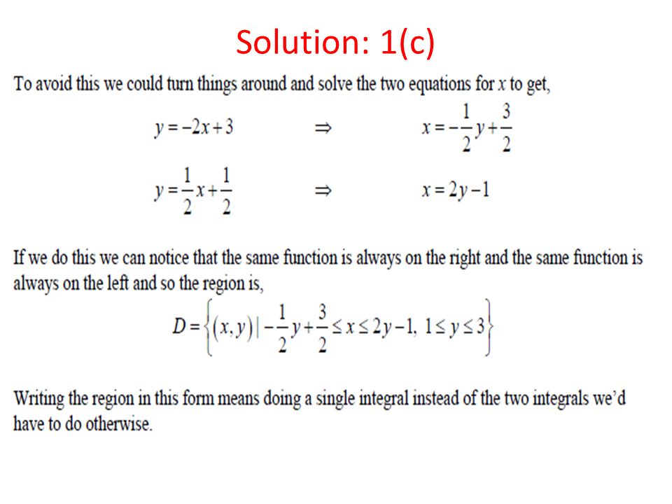
74. Solution: 1(c)

79. Exercise: 1 Evaluate where D is the region bounded by the parabolas y = 2x 2 and y = 1 + x 2.

80. The parabolas intersect when 2x 2 = 1 + x 2, that is, x 2 = 1. – Thus, x = ±1. Exercise: 1 (contd.)

81. We note that the region D is a type I region but not a type II region. – So, we can write: D = {(x, y) | –1 ≤ x ≤ 1, 2x 2 ≤ y ≤ 1 + x 2 } Exercise: 1 (contd.)

82. The lower boundary is y = 2x 2 and the upper boundary is y = 1 + x 2. Exercise: 1 (contd.)

84. When we set up a double integral as in Exercise 1, it is essential to draw a diagram. – Often, it is helpful to draw a vertical arrow as shown. Exercise: 1 (contd.)

85. Then, the limits of integration for the inner integral can be read from the diagram: – The arrow starts at the lower boundary y = g 1 (x), which gives the lower limit in the integral. – The arrow ends at the upper boundary y = g 2 (x), which gives the upper limit of integration. Exercise: 1 (contd.)

86. NOTE For a type II region, the arrow is drawn horizontally from the left boundary to the right boundary.

87. Find the volume of the solid that lies under the paraboloid z = x 2 + y 2 and above the region D in the xy–plane bounded by the line y = 2x and the parabola y = x 2. Exercise: 2

88. From the figure, we see that D is a type I region and D = {(x, y) | 0 ≤ x ≤ 2, x 2 ≤ y ≤ 2x} – So, the volume under z = x 2 + y 2 and above D is calculated as follows. Exercise: 2 (contd.)

91. From this figure, we see that D can also be written as a type II region: D = {(x, y) | 0 ≤ y ≤ 4, ½y ≤ x ≤ – So, another expression for V is as follows. Exercise: 2 (Another way!)

92. Exercise: 2 (contd.)

93. Reversing the order of Integration

94. Example: 1(a)

97. Example: 1(b)