1. Jaypee Institute of Information Technology University, Jaypee Institute of Information Technology University,Noida Department of Physics and materials Science and Engineering

2. Coulombs Law Like charges repel, unlike charges attract. The electric force acting on a point charge q 1 as a result of the presence of a second point charge q 2 is given by Coulomb's Law: where  0 = permittivity of space

4. Gauss's Law The total of the electric flux out of a closed surface is equal to the charge enclosed divided by the permittivity. Electric Flux over a Closed Surface = Charge enclosed by the Surface divided by  o.  o = the permittivity of free space 8.854x10 -12 C 2 /(N m 2 ) = 1/4  k)

5. . A more intuitive statement: the total number of electric field line entering or leaving a closed volume of space is directly proportional to the charge enclosed by the volume If there is no net charge inside some volume of space then the electric flux over the surface of that volume is always equal to zero. Electric Flux: The Electric Flux  E is the product of Component of the Electric Field Perpendicular to a Surface times the Surface Area.

12. Laplace's and Poisson's Equations A useful approach to the calculation of electric potentials is to relate that potential to the charge density which gives rise to it. The electric field is related to the charge density by the divergence relationship and the electric field is related to the electric potential by a gradient relationship

13. Therefore the potential is related to the charge density by Poisson's equation This is Poisson's equation. In a charge-free region of space, this becomes Laplace's equation

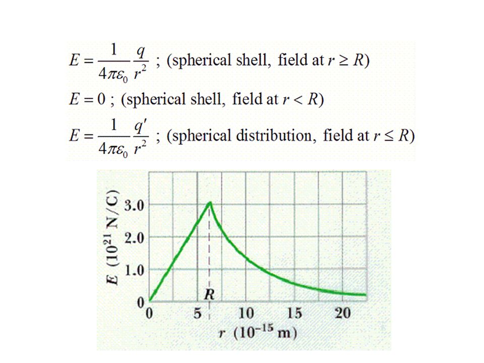
14. Potential of a Uniform Sphere of Charge Since the potential is a scalar function, this approach has advantages over trying to calculate the electric field directly. Once the potential has been calculated, the electric field can be computed by taking the gradient of the potential. The use of Poisson's and Laplace's equations will be explored for a uniform sphere of charge. In spherical polar coordinates, Poisson's equation takes the form:

15. Biot-Savart Law Currents, i.e. moving electric charges, produce magnetic fields. There are no magnetic charges The Biot-Savart Law relates magnetic fields to the currents which are their sources. In a similar manner, Coulomb's law relates electric fields to the point charges which are their sources.

16. where µ 0 is the permeability constant The Biot-Savart Law is used to calculate the magnetic field at a given position. It is usually only practical to do the calculation in special cases where some symmetry makes the problem simpler.

17. Ampere's Law Ampere's law allows us to write down a single equation that describes all of the ways that electric current can make magnetic field. But, just as with Gauss's law, this single equation is very difficult to solve. Ampere's law says: The path integral of around any (imaginary) closed path is equal to the current enclosed by the path, multiplied by When we discussed Gauss's law, we noted that the law was true no matter how distorted the surface or how complicated the electric field. Similarly, Ampere's law is always true,

18. magnetic field around an infinitely long wire But B has the same value a distance a away from the rod and hence

19. Maxwell's Equations Gauss' law in Electrostatics (Source of E) Faraday's law (Source of E) Ampere-Maxwell’s law (Source of B) Gauss' law in Magnetostatics.dl

20. Differential form of Maxwell’s Equations Gauss' law Faraday's law Ampere's law

21. Ampere’s Law (constant currents): Ampere’s Law for constant currents. What about currents which are not continuous? The capacitor holds a charge Q over the two plates. How can there be a current emerging from the capacitor plates? I

22. PHYS 102 Ampere’s Law (continuous currents?): Ampere’s Law for constant currents. I +Q charge deposits on the plate E-field increasing as Q increases! -Q charge induced by E-field I

23. PHYS 102 Ampere’s Law (modification?): Faraday’s Law A changing magnetic flux creates an electric field!!! Ampere’s Law for constant currents. Scottish physicist James Clerk Maxwell suggests that a changing electric flux creates a magnetic field!!!

24. PHYS 102 Ampere’s Law (modification?): Modified Ampere’s Law. Is termed the displacement current.

25. PHYS 102 Modified Ampere’s Law To see how the displacement current comes about, one has to consider the electric flux through the capacitor’s plate (Gauss’s Law). Q increases on the capacitor, the electric flux also increases at the same rate.

26. PHYS 102 Modified Ampere’s Law: I I What does B-field look like in this region?

27. PHYS 102 Modified Ampere’s Law: I What does B-field look like in this region? E-field increasing B-field forms concentric rings with direction given as shown.

28. Electromagnetic Waves Transmission of energy through a vacuum or using no medium is accomplished by electromagnetic waves, caused by the osscilation of electric and magnetic fields. They move at a constant speed of 3x10 8 m/s. Often, they are called electromagnetic radiation, light, or photons Light is not the only example of an electromagnetic wave. Other electromagnetic waves include the microwaves and the radio waves that are broadcast from radio stations. An electromagnetic wave can be created by accelerating charges; moving charges back and forth will produce oscillating electric and magnetic fields, and these travel at the speed of light. It would really be more accurate to call the speed "the speed of an electromagnetic wave", because light is just one example of an electromagnetic wave.

29. Reflection and Transmission at Normal incidence Suppose yz plane forms the boundary between two linear media. A plane wave of frequency ω travelling in The x direction (from left) and polarized along y direction, approaches the interface from left (see figure) In medium 1 following reflected wave travels back -sign in B R is because Poynting vector must aim in the direction of propagation

30. Reflection and Transmission at Normal incidence-2 In medium 2 we get a transmitted wave: At x=o the combined fields to the left E I +E R and B I +B R, must join the fields to the right E T and B T in accordance to the boundary condition. Since there are no components perpendicular to the surface so boundary conditions (i) and (ii) are trivial. However last two yields:

31. Reflection and Transmission at Normal incidence-3 The reflected wave is in phase if v 2 >v 1 and out of phase if v 2 <v 1

32. Reflected wave is 180 o out of phase when reflected from a denser medium. This fact was encountered by you during Last semester optics course. Now you have a proof!!!

33. Reflection coefficient (R) and Transmission coefficient (T) Intensity (average power per unit area is given by): If μ 1 = μ 2 = μ 0, i.e μ r =1, then the ratio of the reflected intensity to the incident intensity is Where as the ratio of transmitted intensity to incident intensity is NOTE: R+T=1 => conservation of energy, Use ε α (n) 2

34. Oblique Incidence