1. Adapted from Rappaport’s Chapter 4 Mobile Radio Propagation: Large-Scale Path Loss
The transmission path between the transmitter and the receiver can vary from simple line-of-sight to one that is severely obstructed by buildings, mountains, and foliage.
Unlike wired channels that are stationary and predictable, radio channels are extremely random and do not offer easy analysis.
Modeling the difficult parts of mobile radio system design, and is typically done in a statistical fashion, based on measurements.

2. 4.1 Introduction to Radio Wave Propagation
The mechanisms behind electromagnetic wave propagation are diverse, but can generally be attributed to reflection, diffraction, and scattering.
Due to multiple reflections from various objects, the electromagnetic waves travel along different paths of varying lengths. The interaction between those waves causes multipath fading at a specific location.

3. Strengths of the waves decrease as the distance between the transmitter and receiver increases.
Propagation models
Large-scale path loss model
Small-scale fading model

4. Large-Scale Path Loss Model
Focus on predicting the average received signal strength at a given distance from the transmitter.
Useful in estimating the coverage area of an antenna.
Typically the local average received power is computed by averaging signal measurements over a measurement track of 5 λto 40λ.
For cellular system in 1~2 GHz, this corresponds to 1~10m

5. Small –scale fading Model
Focus on the variability of the signal strength in close spatial proximity to a particular location.
Characterize the rapid fluctuations of the received signal strength over very short travel distances (a few wavelengths ) or short time durations.
The received power may very by dB when the receiver is moved by only 1 fraction of a wavelength, due to the fact that the received signal is a sum of many contributions (the phases are random) coming from different directions.

6. Figure 4.1 (P.106) illustrates small-scale fading and the slower large-scale variations for an indoor radio communication system.

7. This chapter covers large-scale propagation and presents a number of common methods used to predict received power in mobile comm. sys.
Chap5 treats small-scale fading models and describes methods to measure and model multi-path in the mobile radio environment.

8. 4.2 Free Space propagation Model
Used to predict received signal strength when the transmitter and receiver have a clear, unobstructed line-of- sight path between them.
For examples: Satellite comm. systems and microwave line-of-sight radio links.

9. The power received by a receiver antenna at a distance d is given by the Friis free space equation:
(4.1)
where Pt: transmitted power
Pr: received power
Gt, Gr: antenna gain
L: the system loss factor not related to propagation. (miscellaneous loss, and L 1)
: wavelength in meters

10. The wavelength is related to the carrier frequency (4.3)
The gain of an antenna
(4.2)
where Ae: the effective aperture related to the physical size of antenna.
The wavelength is related to the carrier frequency
(4.3)
where f: the carrier frequency in Hertz
: the carrier frequency in radians per second.
c: the speed of light in meters/sec

11. Equation (4.1) implies that the received power decays with distance at a rate of 20dB/decade.
Isotropic radiator
an ideal antenna which radiates power with unit gain uniformly in all direction.
Often used to reference antenna gains in wireless systems.
Effective isotropic radiated power (EIRP)=PtGt
Represents the maximum radiated power available from a transmitter in the direction of maximum antenna gain, as compared to an isotropic radiator.

12. In practice, effective radiated power (ERP) is used instead of EIRP to denote the maximum radiated power as compared to a half-wave dipole antenna.
Since a dipole antenna has a gain of 1.64 (2.15dB) above an isotropic antenna, the ERP will be 2.15 dB smaller than the EIRP for the same transmission system.
Antenna gains are given in
dBi (dB gain with respect to an isotropic source).
dBd (dB gain with respect to a half-wave dipole).

13. Path Loss (or its reciprocal, received power are the most important parameter predicated by large-scale propagation model.)
Represents signal attenuation in dB between the effective XMIT power and the RCVR power.
For free space
(4.5)
which is valid only in the far-field of transmitting antenna region.
That is, the far-field distance
and df must satisfy
df >>D and df >>
where D is the largest physical linear dimension of antenna.

14. The Equation (4. 1) does not hold for d=0
The Equation (4.1) does not hold for d=0. For this reason, large-scale propagation models use a close-in distance, d0, as a known received power reference point.
The received power, Pr(d), at any distance d>d0, may be related to Pr(d0).
The value Pr(d0) may be predicted from equation (4.1), or may be measured in the radio environment by taking the average received power at many points located at a close-in radial distance d0 from the transmitter.

15. The reference distance must be chosen such that it lies in the far-field region, that is, d0 df, and d0 is chosen to be smaller than any practical distance used in the mobile communication system.
Thus, at a distance greater than d0,
(4.8)
measured in units of dBm or dBW
(4.9)
where Pr(d0) in units of watts.

16. For practical system using low-gain antennas in the 1~2 GHz region,
1m in indoor environments
100m or 1km in outdoor environments.

17. Example 4.1+4.2 (p109-110) for path Loss and Received power.

19. 4.3 Relating Power to Electric Field
A linear radiator

20. It produces electric and magnetic fields (4.10) (4.11) (4.12)
with
where
At far-field region, only the radiated field components are considered.

21. In free space, the power flux density (w/m2) is given by (4.13)
where is the intrinsic impedance of free space and is given by

22. Consequently,
(4.14)
where |E| represents the magnitude of the radiating portion of the electric field in the far field.

23. Figure 4.3a illustrates how the power flux density disperses in free space from an isotropic point source.
Pd may be thought of as the EIRP divided by the surface area of a sphere with radius d.

24. The power received at distance d is given by
(4.15)
relates the Electric field |E| to received power in watts.
Also can be modeled as an equivalent circuit in Figure 4.3b, and the received power is given by
(4.16)

26. 4.4 The three basic mechanisms that impacts propagation
Reflection: electromagnetic wave impinges upon an object which has very large dimensions when compared to the wavelength of the propagation wave.
Occurs from the surface of the earth, building and walls.
Diffraction: occurs when the radio path is obstructed by a surface that has sharp irregularities (edges).
Secondary waves present throughout the space and even behind the obstacles, giving rise to a bending of waves around the obstacles.

27. Scattering: occurs when the medium through which the wave travel consists of objects with dimensions that are small compared to the wavelength, and where the number to obstacles per unit volume is large.
foliage, street signs. Lamp posts.

28. The Fresnel reflection coefficient ( ) is a function of
When an radio wave propagating in one medium impinges upon another medium having different electrical properties, the wave is partially reflected and partially transmitted.
The Fresnel reflection coefficient ( ) is a function of
material properties
wave polarization
angle of incidence
frequency of the propagating wave

29. 4.5.1 Reflection from Dielectrics
Figure 4.4 shows an electromagnetic wave incident at an angle with the plane of the boundary between two dielectric media.

30. The nature of reflection varies with the direction of polarization of the E-field.
The plane of incidence is defined as the plane perpendicular to the boundary surface and containing the incident, reflected, and transmitted rays.
Parameters , , and represent the permittivity, permeability, and conductance of the media, respectively.
Some of them are sensitive to the operating frequency as shown in Table 4.1 (P. 116)

32. Because of superposition, only orthogonal polarizations need be considered to solve general reflection problem. The reflection coefficient
(4.19)
(4.20)
where is the intrinsic impedance of the ith medium and is given by , that is, the radio of electric to magnetic field for a uniform plane wave in the particular medium.

33. The velocity of an electromagnetic wave is given by , and the boundary conditions at the surface of incidence obey Snell’s Law which is given by
(4.21)
(4.22)
and
(4.23a)
(4.23b)

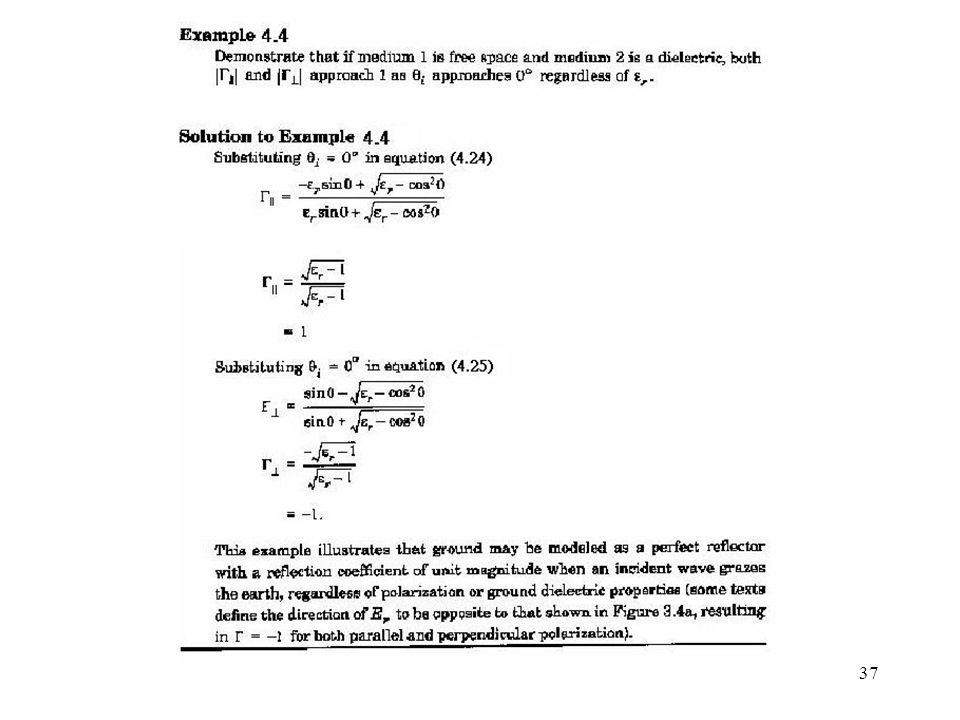
34. For the case when the first medium is free space, the equations (4
For the case when the first medium is free space, the equations (4.19) and (4.20) can be simplified to
(4.24)
(4.25)

35. For the case of elliptical polarized waves, the wave may be broken down to two components as shown in Figure 4.5

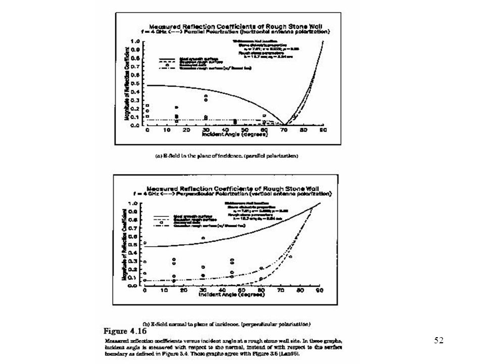
36. Figure 4.6 shows a plot of the reflection coefficient for both horizontal and vertical polarization as a function of the incident angle.

38. The angle at which no reflection occurs in the medium of origin.
4.5.2 Brewster Angle
The angle at which no reflection occurs in the medium of origin.
Occurs only for the vertical polarization.
(4.27) or
(4.28)
if the first medium is free space

40. 4.5.3 Reflection from perfect Conductors
Since electromagnetic energy cannot pass through a perfect conductor a plane wave incident on a conductor has all its energy reflected.
(4.29)
(4.30)
(4.31)
(4.32)
Referring to the equations above, we see that for a perfect conductor, , and , regardless of incident angle.

41. 4.6 Ground Reflection (2-ray) Model
reasonably accurate for predicting the large-scale signal strength for the system that uses tall towers, as well as for Line-of-sight microcell channel.

42. The total received E-field, ETOT, is then a result of the direct line-of-sight component, ELOS, and the ground reflected component, Eg.
where
(4.34)
(4.35)
Then,
(4.39)

43. as d becomes large
(4.51)
(4.52)
(4.53)

45. 4.7 Diffraction 4.7.1 Fresnel Zone Geometry
(4.54)
(4.55)
(4.56)
(4.57)

46. The phase different between a direct LOS path and diffracted path is a fun of height and position of the obstruction, as well as the XMIT and RCVR location.
Fresnel Zones
excess path length :

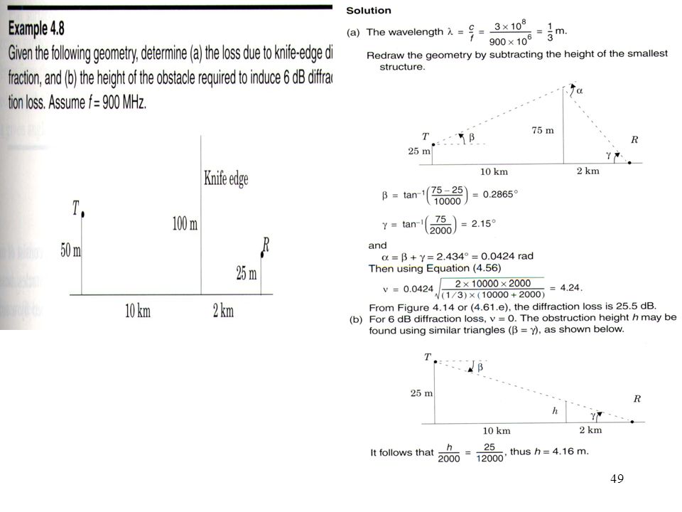
47. 4.7.2 Knife- edge Diffraction Model

50. 4.7.3 Multiple Knife- edge Diffraction

51. surface protuberance for a given angle of incidence :
4.8 Scattering
surface protuberance for a given angle of incidence :
(4.62)
Scattering loss factor
(4.63)
A modified reflection coefficient
(4.65)

53. 4.9 Practical Link Budget Design Using Path Loss Models
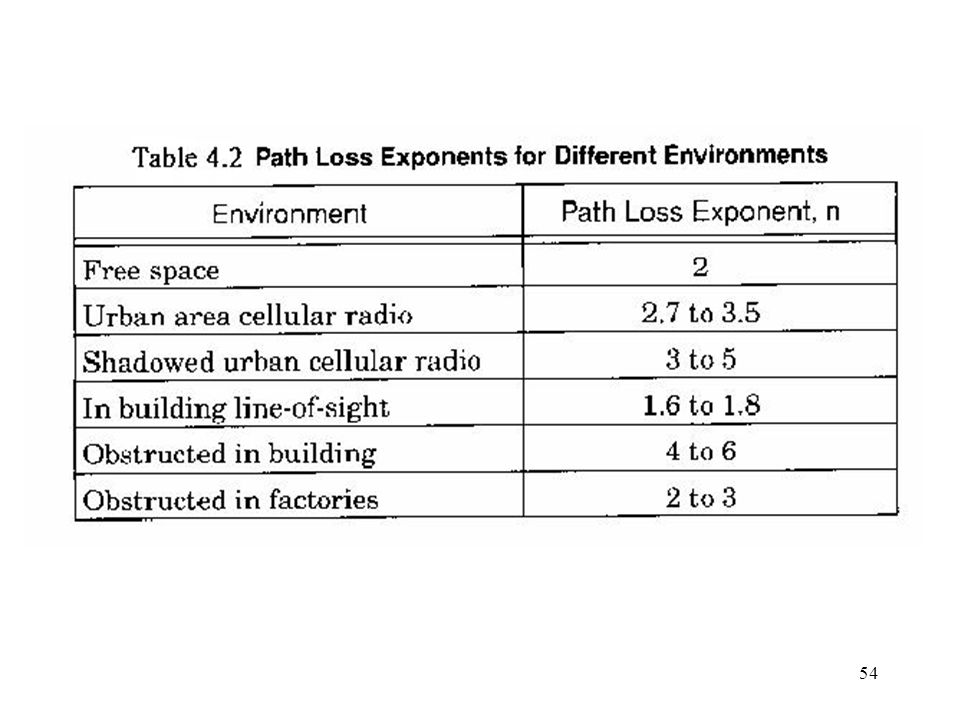
4.9.1 Log-distance Path Loss Model
(4.67) or
(4.68)
where n is the path loss exponent
d0 is the close-in reference distance

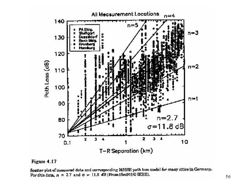
55. 4.9.2 Log-normal shadowing
(4.69a)
where is a zero-mean Gaussian distributed random variable (in dB) with standard deviation (also in dB).
Implies that measured signal levels at a specific T-R separation have a Gaussian (normal) distribution about the distance-dependent mean of (4.68) (Fig4.17 p141)

57. Since PL(d) is a random variable so is Pr(d)
Q-fun or erf fun can be used to determine the probability that the received signal level will exceed (or fall below) a particular level.
(4.70a)
where
(4.70b)
(4.71)
Appendix D

58. 4.9.3 Determination of percentage of coverage Area
percentage of useful service area
(i.e. the percentage of area with a received signed that is equal or greater than r)
(4.73)

59. (4.79)+Fig. 4.18

61. 4.10 Outdoor Propagation Models
The terrain profile of a particular area needs to be taken into account for estimating the path loss.
Most of these models are based on a systematic interpretation of measurement data obtained in the service area.
Okumvra Model etc.

62. 4.11 Indoor Propagation Models differs in two aspects
the distances covered are much smaller
the variability of the environment is greater

63. Partition Losses (same floor)

65. Partition Losses between Floors

67. Log-distance path Loss Model.

68. 4.12 Signal penetration into Buildings
Signal strength received inside a building increases with height.
RF penetration is a fun of frequency as well as height within the building.
, penetration Loss increases due to the shadowing effects of adjacent buildings.

69. 4.13 Ray Tracing + Site Specific Modeling
SIte SPecific (SISP) models
GIS databases