1. Earth resistivity tomography L. Baron 12/04/2012
ERT basics
Earth resistivity tomography
L. Baron
12/04/2012

2. Introduction
Electrical prospecting implies detection on the surface of effects produced by electrical current flow in the ground. There is a large variety of techniques available using electrical methods, we may measure for example:
the electrical potential;
the current;
the magnetic field.
Moreover, the measurements can be made
in a variety of ways. The methods based on
the measure of the parameter "resistivity"
are currently the most developed and the
most diversified.
They were imagined in
1912 by the Schlumberger brothers.

3. Resistivity definition
The resistivity of a material is the physical property which determines the aptitude of this material to be opposed to the passage of the electrical current. The resistivity is the ohmic resistance of a cylinder of unit section and length.
The usual units are the Ohm for resistances and the meter for the lengths. The resistivity unit will be thus the Ohm.m. In hydrogeology we generally employ the microSiemens/cm = 10’000 / Ohm.m

4. Propagation of electrical current
Electrical current may be propagated in rock sand minerals in three ways. By the:
Solid conductibility;
Surface conduction;
Electrolytic conduction.
In fact, in most of the rocks, conductibility is electrolytic type. The current is carried by ions. The electrical resistivity of rocks bearing water is controlled mainly by the water which they contain.
The resistivity of a rock will depend :
On the quality of the electrolyte, i.e. of the resistivity of the natural pore water and consequently the quantity of dissolved salts in the electrolyte;
On the quantity of electrolyte contained in the unit of rock volume;
On the mode of electrolyte distribution.

5. Quality of the electrolyte
When a salt dissolves in water, it dissociates in positively and negatively charged ions. Under the effect of an electrical field, ions will move giving rise to an electrical current. This displacement is obstructed by the viscosity of the water and for a given ion reach a limited velocity called mobility of ions. The conductibility of an electrolyte depends in fact on concentration of ions, mobility of the different ions and degree of dissociation. A water with a same concentration in amount of dissolved salts will have a different resistivity according to involved ions.

6. Salinity
Equivalent salinity is salinity in NaCl which would cause a resistivity equal to that of water considered. It is possible to obtain coefficients which make it possible to pass from various salts to the NaCl equivalent. The reverse is not true, the knowledge of the resistivity of a water only makes it possible to obtain its NaCl equivalent and not its composition.
The quality of a water in a rock will also depend on:
the nature of original water;
the solubility of minerals of the rock;
the age of the rock.
Generally, the rocks with fine grains and fine pores thus contain water more salty, more conductive, than the more permeable rocks, where water does not circulate and take on ions. Thus, the argillaceous moraine contains a water in general much more conductive than that of the gravels. The oldest rocks present more salt charged water.

7. The temperature effect
The resistivity of an electrolyte also depends on the temperature. An increase in temperature decreases viscosity. The mobility of ions becomes larger and dissociation increases, which causes to decrease the resistivity or conversely to increase conductivity.

8. Different waters
From the chemical point of view, we define the dry residue, obtained after filtering and evaporation, which represents the total of the dissolved materials. It is expressed in g/liter. l g/liter = 1000 ppm l mg/liter = 1ppm It is generally admitted that if this dry waste is higher than 8g/liter( 8000 ppm) water is unsuitable for drinking. This limit, somewhat arbitrary, depends on the water resources of the area.

9. Porosity
The quantity of water contained in rocks depends upon porosity.
We can define:
Total porosity
Effective porosity

10. Total porosity
Total porosity is the ratio of the voids volume in the rocks to the total volume of the rock. It is a dimensionless quantity expressed as a percentage. We differentiate between primary and secondary porosity. Primary porosity, created during the deposition of the sediment, is an intergranular type. Its magnitude depends on the degree of sorting and the shape of the grains. It does not depend on the grain size. Primary porosity, which is mainly observed in clastic rocks, generally decreases in time due to the effects of cementation and compaction. Secondary porosity includes porosity acquired as a result of dissolution, fracture porosity and intergranular porosity, due to weathering.

11. Effective porosity
Pores, to allow the circulation of fluid should be connected. Effective porosity can be defined as:
It can be much lower than the total porosity when the pores in a rock are not connected (pumice stone) or when the size of the pores is such that the fluids cannot circulate (silts) or even when a part of the water is absorbed by the minerals in the rock (clay).

12. Archie's law: Definition
The electrical resistivity of a rock depends mainly on quantity of water in a unit volume of rock, and on the quality of this water. These factors are taken into account in the "Archie law" (Archie 1942) which links the resistivity of the rock, the porosity, the nature of distribution and the resistivity of the electrolyte. a: factor which depends of the lithology and varies between 0.6 and 2 (a < 1 for rocks with intergranular porosity and a > 1 for rocks with fractured porosity) m: cementation factor, it depends of the pores shape, of the compaction and varies between 1,3 for unconsolidated sands to 2,2 for cimented limestone. Generally the parameter F is known as Formation Factor

13. Archie's law: Saturation
Archie's Law has been established for saturated rocks, but may also take into account another parameter: the saturation Archie's Law becomes n: Its value is about 2 for majority of the formations with normal porosities containing water between 20 and 100 %. Sometimes the air can be replaced by oil or gas, which has the same effect on the resistivities, these three fluids being infinitely resistant. Generally, the desaturation increases the resistivity. In certain very particular cases the effect of the desaturation can be opposite. Since, evaporation charges out of salts the deshydrated zone, which becomes more conductive than the saturated zone from its great salt concentration, it is the case for example in some Egypt areas.

14. Resistivity and lithology
This technique is based on the measurement from the surface of the apparent resistivities of the ground. The value of its resistivity which can varies:
From 1 to 10 Ohm.m for clay and marl;
From 10 to 100 Ohm.m for sands and sandstone;
From 100 to thousands of Ohm.m for limestone and the eruptive rocks.
The correspondence between the resistivity and the geological facies is a concept of great practical importance. Sometimes, some facies, clays for example, keep practically the same resistivity on hundreds of kilometers; in general, the resistivity of a formation is less constant and can change gradually along a same formation especially in the quaternary deposits.
It should be noted that the resistivities which we measure in prospection are already averages relating to great volumes of formation in place which average are greater since the formations are deeper. It results from what precedes that the measurements of resistivity made on samples are comparable with those of the formations in place only if we consider the average value of a great number of samples.

15. Anisotropy
Often, the resistivities of the rocks depend on the direction of the current that crosses them; we say that they are anisotropic.
This anisotropy can be due to the intimate structure of the rock; the sedimentary formations are generally more resistant in the direction perpendicular to the bedding plane for example. It is called micro-anisotropy.
But for great volume, it can also be a question of an apparent anisotropy, successions of layers alternatively resistant and conductive give a value of resistivity higher perpendicular to layers, in this case we call it macro-anisotropy

16. Punctual current source
The Ohm 's law enables us to envisage the flow of current in a homogeneous and isotropic medium. Considering an homogeneous and isotropic formation of resistivity limited by a plane surface on the side of the air, we send a D.C. current using a specific electrode A. The current flows radially outward in all direction from the point A and will produce variations of potential in the ground because of the ohmic resistance of this one. The distribution of the potential can be represented by half-spherical surfaces centered on A. In an isotropic homogeneous medium the potential V due to a point source decreases proportionally to the distance R, and, in addition proportional to intensity I of the current sent and the resistivity of the medium. If we compare the formation to a half space homogeneous and infinite, the proportionality factor will be equal to 1/2 ; and by applying the Ohm's law to space separating two equipotentials between which exists a tension V we obtain: by integration with : dV = potential difference[V] rho = resistivity of the medium [ohm.m] I = intensity of the current [A] r = radius [m]

17. Source and sink between A and B
In fact in practice, there are two current electrodes. The current sent by A (+) will be collected by B (-), but according to the principle of superposition, the potential in a point M will be the same one if we send independently a current +I by A or a current +I by B. In addition, the laws which govern the propagation of the electrical phenomena are linear, which means that we can algebrically add the potentials created by various sources. The total potential in a point will be Vtot = V1 + V2 for two current poles.

18. Dipole injection
The curves represented on the figure above show the evolution of the potential. The fields V and E are appreciably uniform in the central third part of AB while the major part of the fall of potential is localized in the immediate vicinity of electrodes A (+) and B (-), that means that almost the totality of the resistance which offers the formation to the flow of the current comes from the immediate vicinity of electrodes A and B.
For example for an electrode of diameter a, 90% of the resistance of the circuit is located in a sphere of radius 10a, the remainder of the formation having a very weak contribution, it will be thus impossible to know the nature of the underground by the study of resistance between two points. The deep layers of the basement appear only by their influence on the distribution of the potential to the central third of the configuration, from where we need to measure the potential.

19. Decreasing of current density
The current density versus depth is illustrated by the following: Decreasing of the current (I) with the depth (z), for a spacing between the electrodes of L (from Telford, 1990) We admit that for a homogeneous ground 30% of the current is between the surface and a depth z = AB/4, 50% of the current between the surface and z = AB/2 and 70% of the current between the surface and z = AB . These figures allow to appreciate to what point the emitted current by two surface electrodes penetrate in the underground and can be affected by the rocks located in-depth.

20. Reciprocity
In an unspecified medium, homogeneous or heterogeneous, isotropic or anisotropic, the potential created in a point M by a current sent in A is equal to that which we would measure in A if M became source of emission. This is the reciprocity principle. In practice, the current is sent between two poles A and B and we measure the potential difference between the two points M and N, the principles of superposition and reciprocity learn whereas this potential difference is the same one as that which we would observe between A and B if the current were sent between M and N.

21. Tangent law
The existence of a relatively conducting or resistant mass in the ground will disturb the distribution of the flow lines of current and the equipotential lines. Tangents of angles formed by the flow lines of current with the normal at the boundary will be in the inverse ratio of the resistivities.

22. Homogeneous model
The geological example used for modeling is a sandstone level of resistivity 120 ohm.m.
The distribution of the electrical current is done in a homogeneous way in the formation between the electrodes A and B.

23. Two mediums model The geological example used for modelling shows:
A higher level of clayed sandstone of resistivity 30 Ohm.m.
A lower level of sand of resistivity 200 Ohm.
It is noted that the current concentrates in the higher level of low resistivity

24. Two mediums model The geological example used for modelling shows:
a higher level of gravels of resistivity 200 Ohm.m.
a lower level of sandstone of resistivity 30 Ohm.m.
It is noted that the current concentrates in the lower level of low resistivity.

25. Model of resistant furrow
The geological example used for modelling uses three layers:
A higher level of moraine of resistivity 60 Ohm.m.
A marly-sandstone lower level of resistivity 30 Ohm.m.
A furrow filled with gravels of resistivity 400 Ohm.m
It is noted that the current concentrates around the more resistant furrow.

26. Electrode resistance
These electrodes are generally made of steel stakes. The resistance of passage of the current is located in the immediate vicinity of the electrode
Let us suppose a perfectly conducting metal electrode, and calculate the contact resistance of this electrode:
With
L= length to the center of the electrode [m] r = radius of the electrode [m] R = resistance [ohm] rho = resistivity of the formation [ohm.m]
Let us admit for example for the formation a resistivity of 30 ohms.m. The electrode is inserted of 1 m in the ground and has a radius of 0,02 m. Under these conditions, we obtain a contact resistance of R = 234 ohms.

27. Increasing the current
If the current which passes by these electrodes A and B is too weak we can:
change the electrode and put one of larger diameter.
insert it more deeply.
decrease the resistivity of the soil in the vicinity of the electrode, by pouring salted water for example
We understood whereas it is necessary to measure the potential towards the central third of configuration AB in order to be free from the contact resistance (which does not provide information on the nature of the underground).

28. DC implementation
We can measure the potential difference due to the passage of the current sent between A and B by using an apparatus called potentiometer.
In some cases, the potential difference becomes too small to be suitably measured . This difficulty could be resolved in the following way:
Increasing the sensitivity of the apparatus;
Increasing the distance between M and N lead to increase MN corresponds to increase the potential difference.
However, a large MN becomes very receptive with all kinds of parasitic currents such as:
Variable component of the electrical supplies 50 hertz;
Component 16 hertz coming from the railway lines;
No periodic currents, due to the interlocking of various machines;
Currents due to natural sources, telluric, lightning, etc.

29. Apparent resistivity computation
Having measured the potential difference between M and N and the intensity of the current, we can calculate the resistivity. If the formation is homogeneous and isotropic, we will obtain the true resistivity. If on the other hand, the ground is heterogeneous, we will measure the apparent resistivity, which is a function of the nature of the ground and the dimension of the array used. In fact, to a given length of AMNB corresponds a depth of about constant investigation. Dimensions of the configuration will be thus selected according to the problem to treat.

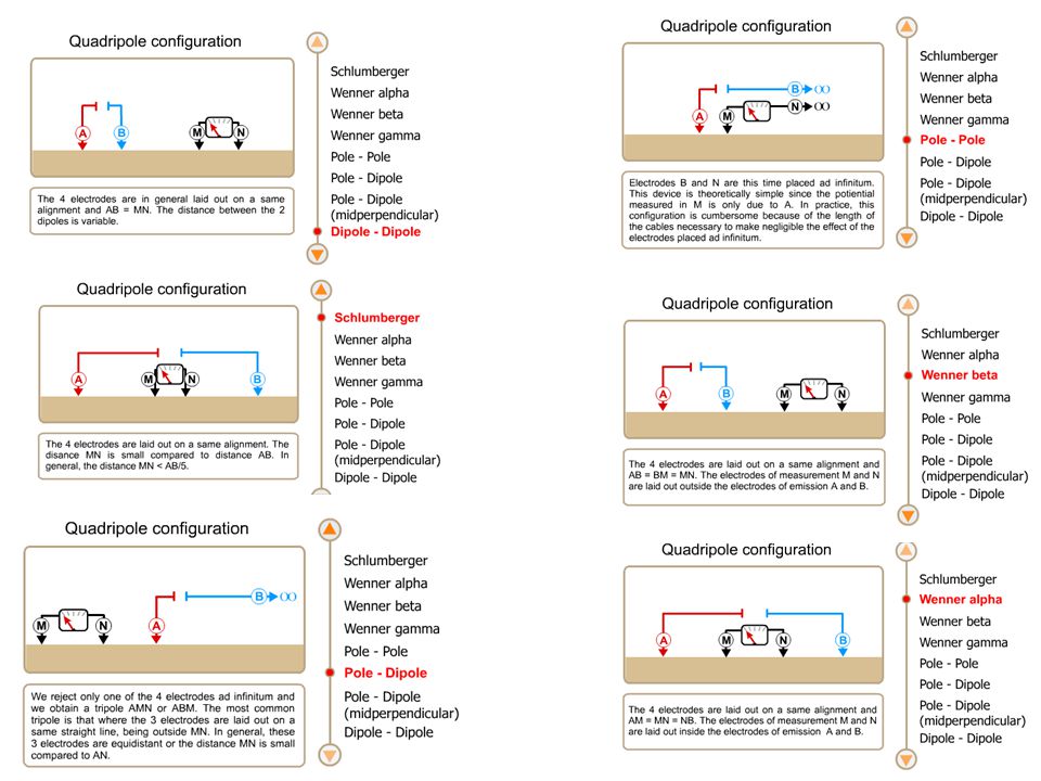
31. Quadripole Configuration
Whatever the array employed, it is characterized by a certain depth of investigation, and resolution. The following table gives for some arrays the depths of investigation and the resolution. It is noticed that resolution and depth of investigation vary in opposite direction. For the dipole-dipole the depth of investigation depends on the spacing between the two most external electrodes.

32. 2D Electrical tomography
The methods of electrical imagery 2D and 3D were developed to obtain a model of the ground where the distribution of resistivities varies vertically and horizontally along the profile. In this case, one supposes that the resistivity does not change in the direction perpendicular to the profile. This assumption is reasonable for many elongated geological bodies and in this case the method could be applied. It will then be necessary to try to place the profiles perpendicular to the body to be studied, what will also enable us to determine the true dimensions of this body.

33. 2D field implementation
A 2D acquisition generally uses a great number of electrodes connected to a multicore cable and placed along a profile. The resistivitymeter is connected to a switch box and automatically selects the electrodes used for the injection of the current and the measurement of the potential. Each electrode has a single numerical address in the configuration, which enables it to be identified by the hardware. The sequence of measurement is generally created in the form of a text file in which is contained various information such as the type of configuration used. The multicore cables are connected to switch boxes. A galvanic contact is ensured with the ground by means of metal stakes (stainless steel). Data is then stored in the memory of the equipment.

34. Acquisition strategy
These are the configurations more often used in electrical imaging tomography.
With:
a: MN [m] separation;
N: data level.

35. Sensibility
The sensitivity function makes it possible to evaluate the influence of a unit volume of the ground on the measured potential difference. The diagram below shows the contour pattern for various arrays. It is immediately noted that the values of this function differ according to the configurations. Each one will have their particular characteristics. This is especially valid at larger distance from the electrodes. The differences in pattern of this function will enable us to better appreciate the response of different arrays to different the types of structures.

36. Median depth
From the sensitivity function we can obtain the median depth of investigation Ze. Ze can be regarded as being the depth at which the upper portion of the earth located at the top of this limit has the same influence as the lower section. This median depth of investigation depends on the configuration used.

37. Apparent resistivity
The figure below presents the electrical tomographies obtained with three different arrays on a model made up of two identical bodies, infinitely long, perpendicular to the array and moved away from four times their width. The patterns generated by these objects strongly differ according to the array employed. This is the reason for which, it is almost impossible to interpret correctly a non- inversed tomography. It is just possible to make some assumptions on the distribution of the apparent resistivities.

38. 2D strategy guidelines
In the presence of a noisy area and without any preliminary knowledge of the geometry of the body studied, it is preferable to use a Wenner-Schlumberger array. This configuration can at the same time be used in geological research on a large scale, hydrogeology, civil engineering, archaeology, and for environmental problems. When we look at vertical structures, and if the area is not too noisy, the resistivimeter rather sensitive, and there is a good ground contact, use a Dipole-Dipole array. This configuration can for example be appropriate in archaeology, mining geophysics and civil engineering. When it is a question of highlighting horizontal structures, if your area is not too noisy and you are short on survey time, use a Wenner array.

39. 3D motivation
Since all geological structures are in 3D in nature, a fully 3D resistivity survey should give better results. A 3D acquisition requires more data and thus costs more. There are however two principal evolutions which currently tend to make the 3D studies possible. It is the recent development of the multichannels resistivimeters which make it possible to take several measurements at the same time, as well as fast evolution of computer software making possible the processing (inversion) of a significant number of data in a reasonable time. The procedure described for 2D acquisitions remains valid in 3D. The electrodes are on the other hand usually arranged according to a square or a rectangle. The shape of the grid can thus vary according to that of the body to study. The interelectrode is also identical according to axes X and Y of the array. One uses primarily Pole-pole, Pole-Dipole and Dipole-Dipole configurations in 3D imaging. The other arrays have weak data coverage towards the edges of the grid.

40. 3D field setup
For small grids (grid lower than 10m by 10m), you can use a Pole-pole because it presents a great variety of combinations and a good horizontal coverage (many points in-depth). It is however sensitive to the noise and has a weak resolution.
Being less sensitive to the noise and presenting a better resolution, the Pole-dipole can be used for larger grids.
A Dipole-Dipole array must be reserved for larger grids (grid higher than 13m by 13m) since it has a weak horizontal coverage compared to a Pole-Pole. A combination of Dipole-Dipole and Pole-Dipole resistivity imaging makes it possible to improve the quality of the results.

41. 2D inversion
The values obtained are apparent resistivities. Measurement represents a value, which integrates the resistivities of a certain volume of the earth. From these values, we want to find the thicknesses and calculated resistivities of the various involved bodies. These calculated resistivities are relatively close to the true resistivities of the bodies.

42. 2D interpretation
The result of a 2D imaging survey is a model presented in the form of pseudosection of the underground. Example of 2D imaging tomography, rock glacier, Verbier, Switzerland.

43. 3D interpretation
For the 3D imaging, the result is presented in the shape of a 3D block. We can also present horizontal and vertical cross-sections of this block "depth slices". The resistivities are in both cases the calculated resistivities.
Example of 3D electrical tomography on an archeological site at Orbe.

44. Conclusion
The result of the inversion is not unique. This non-unicity has several causes. The first comes owing to the fact that the data are often spoilt by errors and that these errors are propagated throughout the inversion process. The second is that the mathematical formalism does not perfectly describe the real physical phenomenon. Moreover, when one uses a least squares minimization criterion, the unicity of the solution will also depends on possible secondary extrema.