Download presentation
Presentation is loading. Please wait.

2
Introduction to Statistics for the Social Sciences SBS200, COMM200, GEOG200, PA200, POL200, or SOC200 Lecture Section 001, Fall, 2014 Room 120 Integrated Learning Center (ILC) 10:00 - 10:50 Mondays, Wednesdays & Fridays. http://www.youtube.com/watch?v=oSQJP40PcGI

3
Hand in your homework & Correlation worksheet

4
Remember: Bring electronic copy of your data (flash drive or email it to yourself) Your data should have correct formatting See Lab Materials link on class website to double- check formatting of excel is exactly consistent Labs
 Your data should have correct formatting See Lab Materials link on class website to double- check formatting of excel is exactly consistent Labs")
5
Schedule of readings Before next exam (September 26 th ) Please read chapters 1 - 4 in Ha & Ha textbook Please read Appendix D, E & F online On syllabus this is referred to as online readings 1, 2 & 3 Please read Chapters 1, 5, 6 and 13 in Plous Chapter 1: Selective Perception Chapter 5: Plasticity Chapter 6: Effects of Question Wording and Framing Chapter 13: Anchoring and Adjustment
 Please read chapters in Ha & Ha textbook Please read Appendix D, E & F online On syllabus this is referred to as online readings 1, 2 & 3 Please read Chapters 1, 5, 6 and 13 in Plous Chapter 1: Selective Perception Chapter 5: Plasticity Chapter 6: Effects of Question Wording and Framing Chapter 13: Anchoring and Adjustment")
6
Reminder A note on doodling

7
By the end of lecture today 9/17/14 Use this as your study guide Characteristics of a distribution Central Tendency Dispersion Primary types of “measures of central tendency”? Mean Median Mode Measures of variability Range Standard deviation Variance Memorizing the four definitional formulae

8
Homework due – Monday (September 22 nd ) On class website: please print and complete homework worksheet # 6 & 7
 On class website: please print and complete homework worksheet # 6 & 7")
9
Overview Frequency distributions The normal curve Mean, Median, Mode, Trimmed Mean Standard deviation, Variance, Range Mean Absolute Deviation Skewed right, skewed left unimodal, bimodal, symmetric Challenge yourself as we work through characteristics of distributions to try to categorize each concept as a measure of 1) central tendency 2) dispersion or 3) shape
 central tendency 2) dispersion or 3) shape")
10
Another example: How many kids in your family? 3 4 8 2 2 1 4 1 14 2 Number of kids in family 1414 3232 1818 4242 214

11
Measures of Central Tendency (Measures of location) The mean, median and mode Mean: The balance point of a distribution. Found by adding up all observations and then dividing by the number of observations Mean for a sample: Mean for a population: ΣX / N = mean = µ (mu) Note: Σ = add up x or X = scores n or N = number of scores Σx / n = mean = x Measures of “location” Where on the number line the scores tend to cluster
 Note: Σ = add up x or X = scores n or N = number of scores Σx / n = mean = x Measures of location Where on the number line the scores tend to cluster.")
12
Measures of Central Tendency (Measures of location) The mean, median and mode Mean: The balance point of a distribution. Found by adding up all observations and then dividing by the number of observations Mean for a sample: Note: Σ = add up x or X = scores n or N = number of scores Σx / n = mean = x Number of kids in family 14 32 18 42 214 41/ 10 = mean = 4.1

13
How many kids are in your family? What is the most common family size? Number of kids in family 13 14 24 28 214 Median: The middle value when observations are ordered from least to most (or most to least)
.")
14
How many kids are in your family? What is the most common family size? Median: The middle value when observations are ordered from least to most (or most to least) 1, 3, 1, 4, 2, 4, 2, 8, 2, 14 1, 2, 3, 4, 8, 14 Number of kids in family 14 32 18 42 214
 1, 3, 1, 4, 2, 4, 2, 8, 2, 14 1, 2, 3, 4, 8, 14 Number of kids in family")
15
Number of kids in family 14 32 18 42 214 14 8, 4, 2, 1, How many kids are in your family? What is the most common family size? Number of kids in family 13 14 24 28 214 Median: The middle value when observations are ordered from least to most (or most to least) 1, 3, 1, 4, 2, 4, 2, 8, 2, 14 2.5 2, 3, 1, 2, 4, 2, 4,8, 1, 14 2, 3, 1, Median always has a percentile rank of 50% regardless of shape of distribution 2 + 3 µ = 2.5 If there appears to be two medians, take the mean of the two
 1, 3, 1, 4, 2, 4, 2, 8, 2, , 3, 1, 2, 4, 2, 4,8, 1, 14 2, 3, 1, Median always has a percentile rank of 50% regardless of shape of distribution µ = 2.5 If there appears to be two medians, take the mean of the two.")
16
Mode: The value of the most frequent observation Number of kids in family 13 14 24 28 214 Score f. 12 23 31 42 50 60 70 81 90 100 110 120 130 141 Please note: The mode is “2” because it is the most frequently occurring score. It occurs “3” times. “3” is not the mode, it is just the frequency for the value that is the mode Bimodal distribution: If there are two most frequent observations

17
What about central tendency for qualitative data? Mode is good for nominal or ordinal data Median can be used with ordinal data Mean can be used with interval or ratio data

18
Overview Frequency distributions The normal curve Mean, Median, Mode, Trimmed Mean Challenge yourself as we work through characteristics of distributions to try to categorize each concept as a measure of 1) central tendency 2) dispersion or 3) shape Skewed right, skewed left unimodal, bimodal, symmetric
 central tendency 2) dispersion or 3) shape Skewed right, skewed left unimodal, bimodal, symmetric")
19
A little more about frequency distributions An example of a normal distribution

20
A little more about frequency distributions An example of a normal distribution

21
A little more about frequency distributions An example of a normal distribution

22
A little more about frequency distributions An example of a normal distribution

23
A little more about frequency distributions An example of a normal distribution

24
Measure of central tendency: describes how scores tend to cluster toward the center of the distribution Normal distribution In a normal distribution: mode = mean = median In all distributions: mode = tallest point median = middle score mean = balance point

25
Measure of central tendency: describes how scores tend to cluster toward the center of the distribution Positively skewed distribution In a positively skewed distribution: mode < median < mean In all distributions: mode = tallest point median = middle score mean = balance point Note: mean is most affected by outliers or skewed distributions

26
Measure of central tendency: describes how scores tend to cluster toward the center of the distribution Negatively skewed distribution In a negatively skewed distribution: mean < median < mode In all distributions: mode = tallest point median = middle score mean = balance point Note: mean is most affected by outliers or skewed distributions

27
Mode: The value of the most frequent observation Bimodal distribution: Distribution with two most frequent observations (2 peaks) Example: Ian coaches two boys baseball teams. One team is made up of 10-year-olds and the other is made up of 16-year-olds. When he measured the height of all of his players he found a bimodal distribution

28
Overview Frequency distributions The normal curve Mean, Median, Mode, Trimmed Mean Standard deviation, Variance, Range Mean Absolute Deviation Skewed right, skewed left unimodal, bimodal, symmetric

29
6’ 7’ 5’ 5’6” 6’6” 6’ 7’ 5’ 5’6” 6’6” 6’ 7’ 5’ 5’6” 6’6” Dispersion: Variability Some distributions are more variable than others Range: The difference between the largest and smallest observations Range for distribution A? Range for distribution B? Range for distribution C? A B C The larger the variability the wider the curve tends to be The smaller the variability the narrower the curve tends to be

31
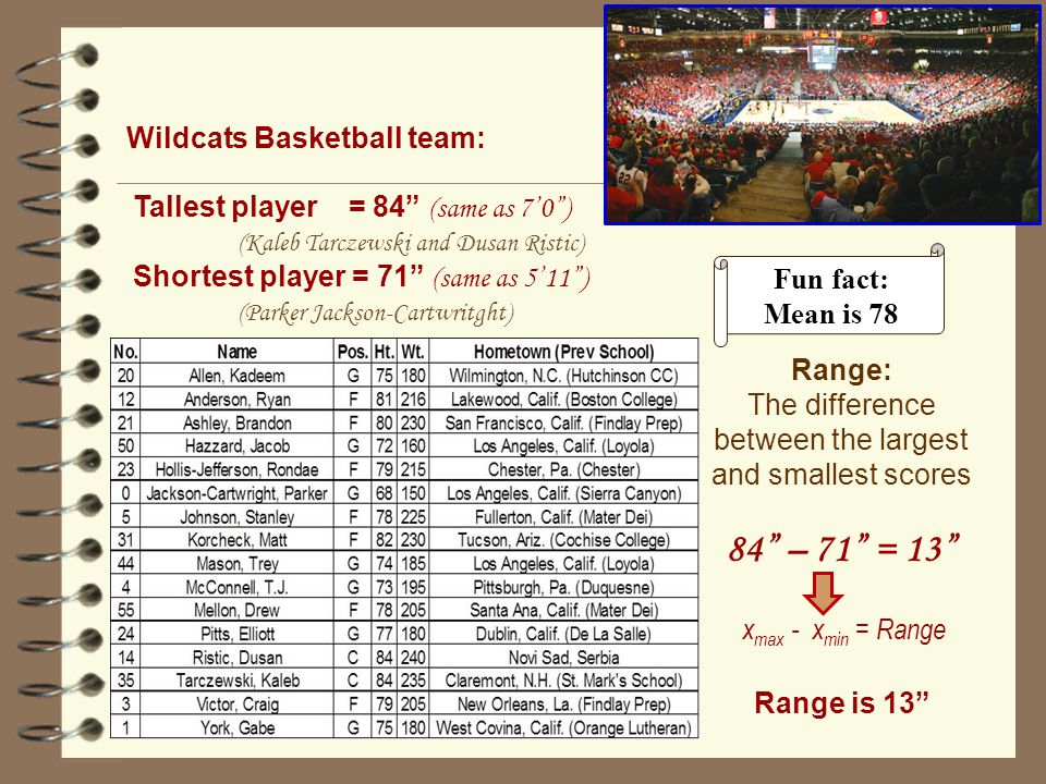
Range: The difference between the largest and smallest scores 84” – 71” = 13” Tallest player = 84” (same as 7’0”) (Kaleb Tarczewski and Dusan Ristic) Shortest player = 71” (same as 5’11”) (Parker Jackson-Cartwritght) Wildcats Basketball team: Range is 13” Fun fact: Mean is 78 x max - x min = Range
 (Kaleb Tarczewski and Dusan Ristic) Shortest player = 71 (same as 5’11 ) (Parker Jackson-Cartwritght) Wildcats Basketball team: Range is 13 Fun fact: Mean is 78 x max - x min = Range")
32
Range: The difference between the largest and smallest score 77” – 70” = 7” Tallest player = 77” (same as 6’5”) (Austin Schnabel) Shortest player = 70” (same as 5’10”) (Five players are 5’10”) Wildcats Baseball team: Range is 7” (77” – 70” ) Fun fact: Mean is 72 x max - x min = Range Please note: No reference is made to numbers between the min and max Baseball
 (Austin Schnabel) Shortest player = 70 (same as 5’10 ) (Five players are 5’10 ) Wildcats Baseball team: Range is 7 (77 – 70 ) Fun fact: Mean is 72 x max - x min = Range Please note: No reference is made to numbers between the min and max Baseball")
33
Frequency distributions The normal curve

34
Variability Some distributions are more variable than others 6’ 7’ 5’ 5’6” 6’6” Let’s say this is our distribution of heights of men on U of A baseball team Mean is 6 feet tall 6’ 7’ 5’ 5’6” 6’6” 6’ 7’ 5’ 5’6” 6’6” What might this be?

35
6’ 7’ 5’ 5’6” 6’6” 6’ 7’ 5’ 5’6” 6’6” 6’ 7’ 5’ 5’6” 6’6” The larger the variability the wider the curve the larger the deviations scores tend to be The smaller the variability the narrower the curve the smaller the deviations scores tend to be Variability

36
Standard deviation: The average amount by which observations deviate on either side of their mean Mean is 6’ Generally, (on average) how far away is each score from the mean?
 how far away is each score from the mean")
37
Let’s build it up again… U of A Baseball team Diallo Diallo is 6’0” Diallo is 0” Deviation scores 6’0” – 6’0” = 0 5’8” 5’10” 6’0” 6’2” 6’4” Diallo’s deviation score is 0

38
Preston Preston is 6’2” 6’2” – 6’0” = 2 5’8” 5’10” 6’0” 6’2” 6’4” Diallo is 0” Preston is 2” Deviation scores Preston’s deviation score is 2” Diallo is 6’0” Diallo’s deviation score is 0 Let’s build it up again… U of A Baseball team

39
Mike Hunter Mike is 5’8” Hunter is 5’10” 5’8” – 6’0” = -4 5’10” – 6’0” = -2 5’8” 5’10” 6’0” 6’2” 6’4” Diallo is 0” Mike is -4” Hunter is -2 Preston is 2” Deviation scores Preston is 6’2” Preston’s deviation score is 2” Diallo is 6’0” Diallo’s deviation score is 0 Mike’s deviation score is -4” Hunter’s deviation score is -2” Let’s build it up again… U of A Baseball team

40
David Shea Shea is 6’4” David is 6’ 0” 6’4” – 6’0” = 4 6’ 0” – 6’0” = 0 5’8” 5’10” 6’0” 6’2” 6’4” Diallo is 0” Mike is -4” Hunter is -2 Shea is 4 David is 0” Preston is 2” Deviation scores Preston’s deviation score is 2” Diallo’s deviation score is 0 Mike’s deviation score is -4” Hunter’s deviation score is -2” Shea’s deviation score is 4” David’s deviation score is 0 Let’s build it up again… U of A Baseball team

41
David Shea 5’8” 5’10” 6’0” 6’2” 6’4” Diallo is 0” Mike is -4” Hunter is -2 Shea is 4 David is 0” Preston is 2” Deviation scores Preston’s deviation score is 2” Diallo’s deviation score is 0 Mike’s deviation score is -4” Hunter’s deviation score is -2” Shea’s deviation score is 4” David’s deviation score is 0” Let’s build it up again… U of A Baseball team

42
5’8” 5’10” 6’0” 6’2” 6’4” Diallo is 0” Mike is -4” Hunter is -2 Shea is 4 David is 0” Preston is 2” Deviation scores Let’s build it up again… U of A Baseball team

43
Standard deviation: The average amount by which observations deviate on either side of their mean 5’8” 5’10” 6’0” 6’2” 6’4” Diallo is 0” Mike is -4” Hunter is -2 Shea is 4 David is 0” Preston is 2” Deviation scores

44
Standard deviation: The average amount by which observations deviate on either side of their mean 5’8” 5’10” 6’0” 6’2” 6’4” Diallo is 0” Mike is -4” Hunter is -2 Shea is 4 David is 0” Preston is 2” Deviation scores

45
Standard deviation: The average amount by which observations deviate on either side of their mean 5’8” 5’10” 6’0” 6’2” 6’4” Diallo is 0” Mike is -4” Hunter is -2 Shea is 4 David is 0” Preston is 2” Deviation scores

46
How do we find the average height? 5’8” - 6’0” = - 4” 5’9” - 6’0” = - 3” 5’10’ - 6’0” = - 2” 5’11” - 6’0” = - 1” 6’0” - 6’0 = 0 6’1” - 6’0” = + 1” 6’2” - 6’0” = + 2” 6’3” - 6’0” = + 3” 6’4” - 6’0” = + 4” Standard deviation: The average amount by which observations deviate on either side of their mean Σ(x - x) = 0 Σ (x - µ ) = ? Diallo Mike Hunter Preston 5’8” 5’10” 6’0” 6’2” 6’4” Diallo is 0” Mike is -4” Hunter is -2 Shea is 4 David is 0” Preston is 2” Deviation scores Σ(x - µ ) = 0 = average height N ΣxΣx = average deviation Σ(x - µ ) N How do we find the average spread?
 = 0 Σ (x - µ ) = . Diallo Mike Hunter Preston 5’8 5’10 6’0 6’2 6’4 Diallo is 0 Mike is -4 Hunter is -2 Shea is 4 David is 0 Preston is 2 Deviation scores Σ(x - µ ) = 0 = average height N ΣxΣx = average deviation Σ(x - µ ) N How do we find the average spread .")
47
5’8” - 6’0” = - 4” 5’9” - 6’0” = - 3” 5’10’ - 6’0” = - 2” 5’11” - 6’0” = - 1” 6’0” - 6’0 = 0 6’1” - 6’0” = + 1” 6’2” - 6’0” = + 2” 6’3” - 6’0” = + 3” 6’4” - 6’0” = + 4” Standard deviation: The average amount by which observations deviate on either side of their mean Σ(x - x) = 0 Σ x - x = ? 5’8” 5’10” 6’0” 6’2” 6’4” Diallo is 0” Mike is -4” Hunter is -2 Shea is 4 David is 0” Preston is 2” Deviation scores Σ(x - µ ) = 0 Big problem Σ(x - x) 2 Square the deviations Σ(x - µ ) 2 N ΣxΣx N Big problem 2
 = 0 Big problem Σ(x - x) 2 Square the deviations Σ(x - µ ) 2 N ΣxΣx N Big problem 2.")
48
Mean: The average value in the data Standard deviation: The average amount scores deviate on either side of their mean Standard deviation is typical “spread” (typical size of deviations or distance from mean) – can never be negative Mean is a measure of typical “value” (where the typical scores are positioned on the number line)
 – can never be negative Mean is a measure of typical value (where the typical scores are positioned on the number line)")
49
Standard deviation: The average amount by which observations deviate on either side of their mean These would be helpful to know by heart – please memorize these formula

50
Standard deviation: The average amount by which observations deviate on either side of their mean What do these two formula have in common?

51
Standard deviation: The average amount by which observations deviate on either side of their mean What do these two formula have in common? n-1 is “Degrees of Freedom” More, next lecture

Similar presentations


 or Ch. 3 (2/3e)>")


