2. To view a full-screen figure during a class, click the red “expand” button.
To return to the previous slide, click the red “shrink” button.
To advance to the next slide, click anywhere on the full screen figure.

3. In 2007, the federal government spent 15 cents of each dollar Canadians earned and collected 16 cents of each dollar earned in taxes.
So the government planned a surplus of 1 cent on every dollar earned.
How does the government’s planned surplus affect the economy?
For many years the federal government had a large deficit and ran up debt.
What are the effects of an ongoing government deficit and accumulating debt?

4. Government Budgets
The federal budget is the annual statement of the federal government’s outlays and tax revenues.
The federal budget has two purposes:
1. To finance the activities of the federal government
2. To achieve macroeconomic objectives
Fiscal policy is the use of the federal budget to achieve macroeconomic objectives, such as full employment, sustained economic growth, and price level stability.

5. Government Budgets Budget Making
The federal government and Parliament make fiscal policy.
After a long, draw-out process of consultations, the Minister of Finance presents a budget plan to Parliament.
Parliament debates the plan and enacts the laws necessary to implement it.

6. Government Budgets Highlights of the 2008 Budget
The projected fiscal 2008 federal budget has revenues of $242 billion, outlays of $240 billion, and a projected deficit of $2 billion.
Revenues come from personal income taxes, corporate income taxes, indirect taxes, and investment income.
Personal income taxes are the largest revenue source.
Outlays are transfer payments, expenditure on goods and services, and debt interest.
Transfer payments are the largest item of outlays.

8. Government Budgets Budget Balance
The federal government’s budget balance equals revenue minus outlays.
If revenues exceed outlays, the government has a budget surplus.
If outlays exceed revenues, the government has a budget deficit.
If revenues equal outlays, the government has a balanced budget.
The projected budget surplus in 2008 of $2 billion.

9. Government Budgets The Budget in Historical Perspective
Figure 29.1 shows the government’s revenues, outlays, and budget balance as a percentage of GDP for the period 1961 to 2007.
As outlays grew and revenues fell, the government deficit increased and peaked at 6.6 percent of GDP in 1985.
During the 1990s, spending cuts eliminated the busget deficit.
In 1997, a budget surplus emerged.

10. Government Budgets

12. Government Budgets Revenues
Figure 29.2 shows revenues as a percentage of GDP.

14. Government Budgets Outlays
Figure 29.3 shows outlays as a percentage of GDP.

16. Government Budgets Deficit and Debt
Government debt is the total amount that the government borrowing. It is the sum of past deficits minus past surpluses.
Figure 29.4 shows the federal government’s debt as a percentage of GDP.
Deficit and debt. Many students need help with the distinction between the deficit and the debt (and with what happens to the debt when there is a surplus). Use the student loan or credit card analogy. Explain that the budget balance—the deficit or surplus—is just like a personal budget balance—the amount that a student borrows or pays back during a given year. The debt—the amount owed by the government—is like the balance on a student loan or credit card account. Students (usually) have a budget deficit and increasing debt. And graduates with a job (usually) have a budget surplus and decreasing debt.
Does the debt matter? You can have endless fun debating this question. If you do engage your students in this question, you will want to point them to thinking about:
1. The distinction between domestically held debt and foreign held debt.
2. No matter how much the government owes every single year, Y = C + I + G + X – M, so the resources available depend on productive capacity, not on paper claims.

18. The Supply-Side Effects of Fiscal Policy
Fiscal policy has important effects on employment, potential GDP, and aggregate supply—called supply-side effects.
An income tax changes full employment and potential GDP.

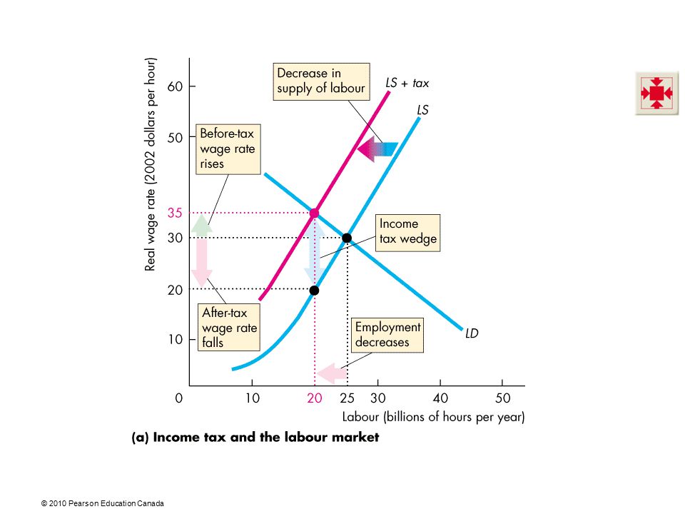
19. The Supply-Side Effects of Fiscal Policy
Full Employment and Potential GDP
Figure 29.5(a) illustrates the effects of an income tax in the labour market.
The supply of labour decreases because the tax decreases the after-tax wage rate.
This section builds on the micro chapters that discuss the effects of taxes. If your students have not yet done a micro course and you want to cover this material, you’ll need to take it slowly and carefully.

21. The Supply-Side Effects of Fiscal Policy
The before-tax real wage rate rises but the after-tax real wage rate falls.
The gap created between the before-tax and after-tax wage rates is called the tax wedge.
The quantity of labour employed decreases.

22. The Supply-Side Effects of Fiscal Policy
When the quantity of labour employed decreases, …
potential GDP decreases.
The supply-side effect of a rise in the income tax decreases potential GDP and decreases aggregate supply.

24. The Supply-Side Effects of Fiscal Policy
Taxes on Expenditure and the Tax Wedge
Taxes on consumption expenditure add to the tax wedge.
The reason is that a tax on consumption raises the prices paid for consumption goods and services and is equivalent to a cut in the real wage rate.
If the income tax rate is 25 percent and the tax rate on consumption expenditure is 10 percent, a dollar earned buys only 65 cents worth of goods and services.
The tax wedge is 35 percent.

25. The Supply-Side Effects of Fiscal Policy
Taxes and the Incentive to Save
A tax on capital income lowers the quantity of saving and investment and slows the growth rate of real GDP.
The interest rate that influence saving and investment is the real after-tax interest rate.
The real after-tax interest rate subtracts the income tax paid on interest income from the real interest.
Taxes depend on the nominal interest rate. So the true tax on interest income depends on the inflation rate.

26. The Supply-Side Effects of Fiscal Policy
Figure 29.6 illustrates the effects of a tax on capital income.
A tax decreases the supply of loanable funds …
a tax wedge is driven between the real interest rate and the real after-tax interest rate.
Investment and saving decrease.

28. The Supply-Side Effects of Fiscal Policy
Tax Revenues and the Laffer Curve
The relationship between the tax rate and the amount of tax revenue collected is called the Laffer curve.
At the tax rate T*, tax revenue is maximized.

30. The Supply-Side Effects of Fiscal Policy
For a tax rate below T*, a rise in the tax rate increases tax revenue.
For a tax rate above T*, a rise in the tax rate decreases tax revenue.

31. Stabilizing the Business Cycle
Fiscal policy actions that seek to stabilize the business cycle work by changing aggregate demand.
■ Discretionary or
■ Automatic
Discretionary fiscal policy is a policy action that is initiated by an act of Parliament.
Automatic fiscal policy is a change in fiscal policy triggered by the state of the economy.

32. Stabilizing the Business Cycle
The Government Expenditure Multiplier
The government expenditure multiplier is the magnification effect of a change in government expenditure on goods and services on aggregate demand.
A multiplier exists because government expenditure is a component of aggregate expenditure.
An increase in government expenditure increases income, which induces additional consumption expenditure and which in turn increases aggregate demand.

33. Stabilizing the Business Cycle
The Autonomous Tax Multiplier
The autonomous tax multiplier is the magnification effect a change in autonomous taxes on aggregate demand.
A decrease in autonomous taxes increases disposable income, which increases consumption expenditure and increases aggregate demand.
The magnitude of the autonomous tax multiplier is smaller than the government expenditure multiplier because the a $1 tax cut induces less than a $1 increase in consumption expenditure.

34. Stabilizing the Business Cycle
The Balanced Budget Multiplier
The balanced tax multiplier is the magnification effect on aggregate demand of a simultaneous change in government expenditure and taxes that leaves the budget balance unchanged.
The balanced budget multiplier is positive because a $1 increase in government expenditure increases aggregate demand by more than a $1 increase in taxes decreases aggregate demand.
So when both government expenditure and taxes increase by $1, aggregate demand increases.

35. Stabilizing the Business Cycle
Discretionary Fiscal Stabilization
Figure 29.8 shows how fiscal policy might close a recessionary gap.
An increase in government expenditure or a tax cut increases aggregate demand.
The multiplier process increases aggregate demand further.

37. Stabilizing the Business Cycle
Figure 29.9 shows how fiscal policy might close an inflationary gap.
A decrease in government expenditure or a tax increase decreases aggregate demand.
The multiplier process decreases aggregate demand further.

39. Stabilizing the Business Cycle
Limitations of Discretionary Fiscal Policy
The use of discretionary fiscal policy is seriously hampered by three time lags:
Recognition lag—the time it takes to figure out that fiscal policy action is needed.
Law-making lag—the time it takes Parliament to pass the laws needed to change taxes or spending.
Impact lag—the time it takes from passing a tax or spending change to its effect on real GDP being felt.
Fiscal policy in practice. Most economists acknowledge that, in principle, discretionary fiscal policy can be used for stabilization purposes, but in practice such stabilization is extremely difficult because of long legislative lags. It is worth reminding the students that the equilibrium in the AS-AD model takes time to work out. The multiplier is a long, drawn-out process. An increase in government expenditure shifts the AD curve rightward, but the new equilibrium price level and real GDP take time to occur. It is also useful to discuss the differences between the potential of fiscal policy under a parliamentary system and under the more rigid U.S. system; the length of time it took the U.S. Congress to pass the 2002 ‘stimulus’ package, compared to almost immediate executive-initiated changes to fiscal policy in Britain, make the point that discretionary fiscal policy is feasible under some governmental systems but only in extreme circumstances in the world’s largest economy.

40. Stabilizing the Business Cycle
Automatic Stabilizers
Automatic stabilizers are mechanisms that stabilize real GDP without explicit action by the government.
Induced taxes and needs-tested spending are automatic stabilizers.
Taxes that vary with real GDP are called induced taxes.
In an expansion, real GDP rises, and wages and profits rise, so the taxes on these incomes—induced taxes—rise.
In a recession, real GDP decreases, wages and profits fall, so the induced taxes on these incomes fall.

41. Stabilizing the Business Cycle
The spending on programs that pay benefits to suitably qualified people and businesses are called transfer payments.
When the economy is in a recession, unemployment is high and transfer payments increase.
When the economy expands, unemployment falls and transfer payments decrease.
Induced taxes and transfer payments decrease the multiplier effects of changes in autonomous expenditure.
So they moderate both expansions and recessions and make real GDP more stable.

42. Stabilizing the Business Cycle
Budget Deficit Over the Business Cycle
Figure 29.10(a) shows business cycle and
Fig (b) shows the budget balance.
The recessions are highlighted.
During a recession, the budget deficit increases.

44. Stabilizing the Business Cycle
Cyclical and Structural Balances
The structural surplus or deficit is the budget balance that would occur if the economy were at full employment and real GDP were equal to potential GDP.
The cyclical surplus or deficit is the actual surplus or deficit minus the structural surplus or deficit.
That is, a cyclical surplus or deficit is the surplus or deficit that occurs purely because real GDP does not equal potential GDP.
Cyclical and structural budget balances. Cyclical and structural budget balances are a difficult concept for many students, but important because of the appropriate measure of fiscal stance.
An effective way to help students see that revenues and outlays will vary as depicted in Figure is to remind them that potential GDP corresponds to full employment, and employment (and so the number of tax payers and recipients of unemployment compensation) changes when real GDP varies.

45. Stabilizing the Business Cycle
Figure illustrates the distinction between a structural and cyclical surplus and deficit.
In part (a), potential GDP is $1,200 billion.
As real GDP fluctuates around potential GDP, a cyclical deficit or cyclical surplus arises.

47. Stabilizing the Business Cycle
In part (b), if real GDP and potential GDP are $1,100 billion, the budget deficit is a structural deficit.
If real GDP and potential GDP are $1,200 billion, the budget is balanced.
If real GDP and potential GDP are $1,300 billion, the budget surplus is a structural surplus.