2. U.S. INFLATION, UNEMPLOYMENT, AND BUSINESS CYCLE29
U.S. INFLATION,
UNEMPLOYMENT,
AND BUSINESS CYCLE

3. Notes and teaching tips: 6, 15, 29, 41, 50, 53, and 56.
To view a full-screen figure during a class, click the red “expand” button.
To return to the previous slide, click the red “shrink” button.
To advance to the next slide, click anywhere on the full screen figure.

4. Inflation Cycles we distinguish two sources of inflation:
Demand-pull inflation
Cost-push inflation

5. Inflation Cycles Demand-Pull Inflation
An inflation that starts because aggregate demand increases is called demand-pull inflation.
Demand-pull inflation can begin with any factor that increases aggregate demand.
Examples are a cut in the interest rate, an increase in the quantity of money, an increase in government expenditure, a tax cut, an increase in exports, or an increase in investment stimulated by an increase in expected future profits.
The potential difficulty with both demand-pull and cost-push inflation stories is how the one-time increase translates into an inflationary process. It is relatively easy to come up with stories as to why aggregate demand might shift continuously to the right, for example because of persistent and growing government budget deficits. What is a little harder is to provide a plausible story as to why the monetary authorities would continue to accommodate this with continuous increases in the quantity of money. Point out that this has been rare in the United States, and has tended to happen when the political situation was such that the Fed was not willing to be blamed for an increase in unemployment. In other countries, particularly where the central bank is less independent than the Fed, it has been more common.

6. Inflation Cycles Initial Effect of an Increase in Aggregate Demand
Figure 29.1(a) illustrates the start of a demand-pull inflation.
Starting from full employment, an increase in aggregate demand shifts the AD curve rightward.

8. Inflation Cycles
The price level rises, real GDP increases, and an inflationary gap arises.
The rising price level is the first step in the demand-pull inflation.

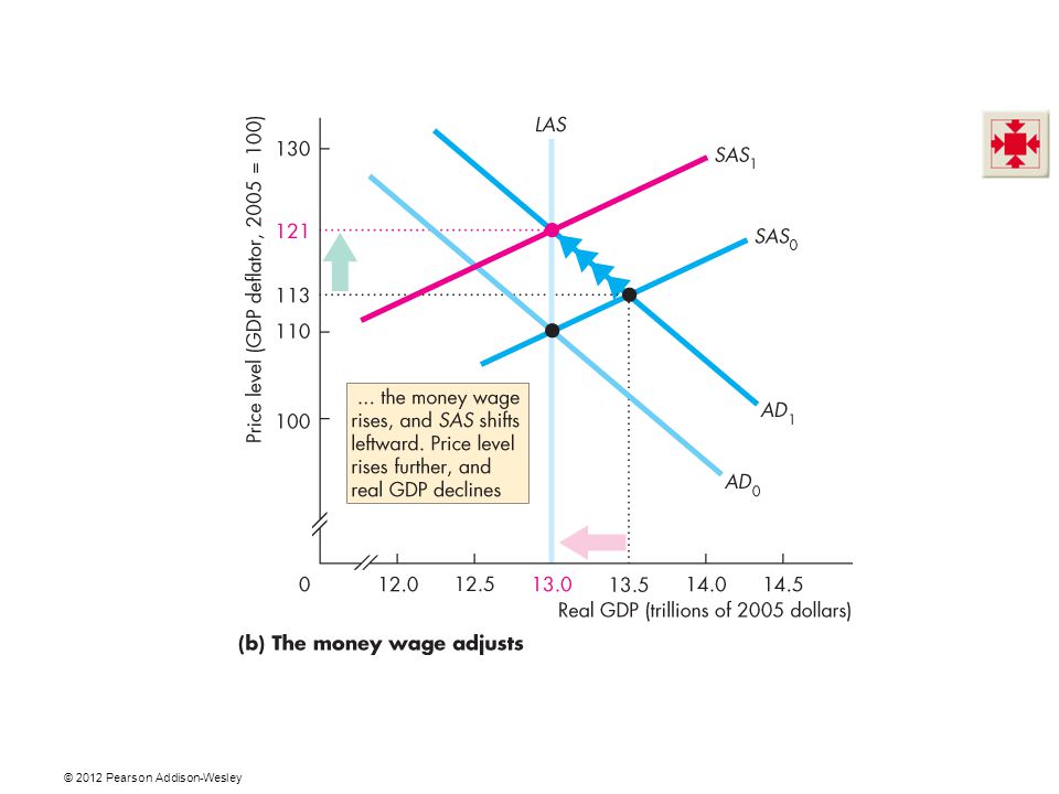
9. Inflation Cycles Money Wage Rate Response
The money wage rate rises and the SAS curve shifts leftward.
The price level rises and real GDP decreases back to potential GDP.

11. Inflation Cycles A Demand-Pull Inflation Process
Figure 29.2 illustrates a demand-pull inflation spiral.
Aggregate demand keeps increasing and the process just described repeats indefinitely.

13. Inflation Cycles
Although any of several factors can increase aggregate demand to start a demand-pull inflation, only an ongoing increase in the quantity of money can sustain it.
Demand-pull inflation occurred in the United States during the late 1960s.

14. Inflation Cycles Cost-Push Inflation
An inflation that starts with an increase in costs is called cost-push inflation.
There are two main sources of increased costs:
1. An increase in the money wage rate
2. An increase in the money price of raw materials, such as oil
The text gives a good description of the first oil price increase in the 1970s as a cost-push inflation, and contrasts it well with the Fed’s refusal to accommodate the second oil price increase in An explanation of how cost-push can be a more widespread cause of inflation in other countries can be given in terms of countries where labor is highly unionized, and in effect there are attempts by different interest groups to obtain shares of GDP that add up to more than 100 percent, with accommodation by a weak monetary authority. Such a process of repeated wage increases, inflation, and monetary accommodation can give rise to continuing inflation. Analysts often “explain” the cause of inflation by focusing attention on the good or service whose price increased the most during the most recent time period. This is incorrect; inflation is cased by monetary growth. One way to point out the fallacy is to use a baseball analogy. Several years ago the average number of home runs hit during major league baseball games increased. Virtually every commentator asked whether the ball had been doctored to make it livelier. No one explained the additional home runs by saying “home runs are higher because Parkin is hitting more home runs than last year.” To explain inflation, economists are looking for an explanation similar to the “doctored ball” explanation of the additional home runs, not an explanation that focuses on the performance of specific players.

15. Inflation Cycles Initial Effect of a Decrease in Aggregate Supply
Figure 29.3(a) illustrates the start of cost-push inflation.
A rise in the price of oil decreases short-run aggregate supply and shifts the SAS curve leftward.
Real GDP decreases and the price level rises.

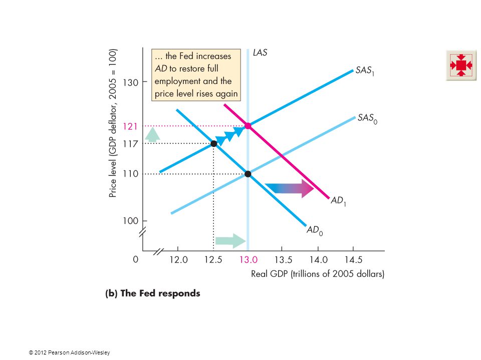
17. Inflation Cycles Aggregate Demand Response
The initial increase in costs creates a one-time rise in the price level, not inflation.
To create inflation, aggregate demand must increase.
That is, the Fed must increase the quantity of money persistently.

18. Inflation Cycles
Figure 29.3(b) illustrates an aggregate demand response.
Real GDP increases and the price level rises again.

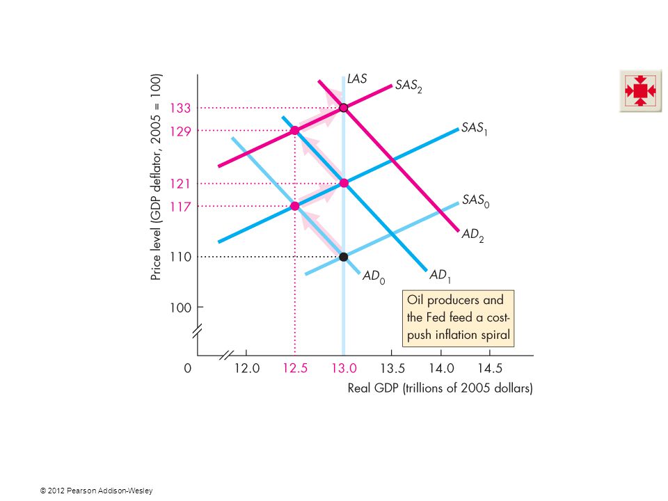
20. Inflation Cycles A Cost-Push Inflation Process
If the oil producers raise the price of oil to try to keep its relative price higher,
and the Fed responds by increasing the quantity of money,
a process of cost-push inflation continues.

22. Inflation Cycles
The combination of a rising price level and a decreasing real GDP is called stagflation.
Cost-push inflation occurred in the United States during the 1970s when the Fed responded to the OPEC oil price rise by increasing the quantity of money.

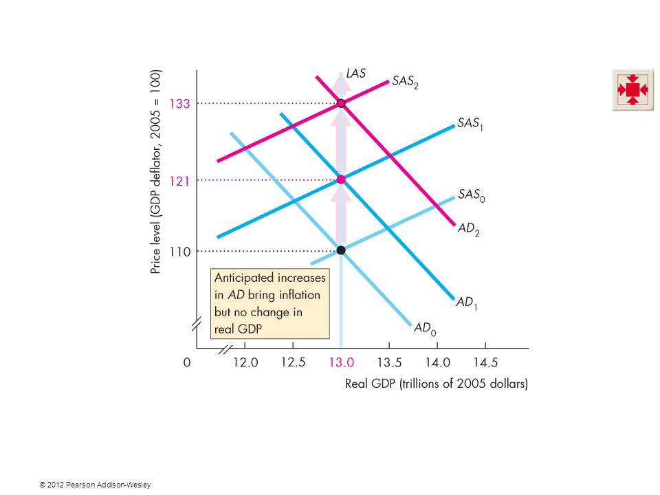
23. Inflation Cycles Expected Inflation
Figure 29.5 illustrates an expected inflation.
Aggregate demand increases, but the increase is expected, so its effect on the price level is expected.

25. Inflation Cycles
The money wage rate rises in line with the expected rise in the price level.
The AD curve shifts rightward and the SAS curve shifts leftward …
so that the price level rises as expected and real GDP remains at potential GDP.

26. Inflation Cycles Forecasting Inflation
To expect inflation, people must forecast it.
The best forecast available is one that is based on all the relevant information and is called a rational expectation.
A rational expectation is not necessarily correct, but it is the best available.

27. Inflation and Unemployment: The Phillips Curve
A Phillips curve is a curve that shows the relationship between the inflation rate and the unemployment rate.
There are two time frames for Phillips curves:
The short-run Phillips curve
The long-run Phillips curve
The Phillips curve story nicely illustrates how progress is made in economics.
The story starts in 1958 when Bill Phillips published his famous paper. At that time the mainstream economic model was the aggregate expenditure model presented in Chapter 25. The model was based on the assumption that the price level was constant, making the inflation rate zero. This assumption was not too unrealistic immediately after World War II. By 1955, though, the inflation rate began to creep higher and averaged 2.7 percent per year between 1956 and Inflation was beginning to be perceived as a problem, one that a model with a “fixed price level assumption” was poorly suited to solve.
In this environment, economists gladly welcomed the simple, short-run Phillips curve, for it gave them a handle on inflation. They believed that they could predict the unemployment rate from their standard model and then combine this unemployment rate with the Phillips curve to determine the resulting inflation rate. The vital assumption in this procedure is that the Phillips curve captures a fixed tradeoff between the actual inflation rate and the unemployment rate that is part of the economy’s structure.
This type of analysis reached its peak of popularity during the early and middle 1960s.
But by 1967 it was under attack. On a theoretical level, Ned Phelps and Milton Friedman pointed out the flimsy justification behind the simple, fixed Phillips curve assumption. On an empirical level, the fixed Phillips curve failed as the inflation rate rose toward the end of the 1960s and into the 1970s: the unemployment rate did not fall as predicted by the fixed Phillips curve.
At this point the idea of a long-run Phillips curve (as distinct from the short-run one) was developed. The concept that aggregate supply is an important component of macroeconomics was taking hold, as was the idea that short-run Phillips curves shift because of changes in people’s expectations. Thus the profession advanced significantly between the initial discussion of the Phillips curve and what students learn today. This advance was the result of the interaction between theory, suggesting that the idea of a fixed short-run Phillips curve was inadequate, and empirical work that reinforced the point that the simple, early approach was deficient.

28. Inflation and Unemployment: The Phillips Curve
The Short-Run Phillips Curve
The short-run Phillips curve shows the tradeoff between the inflation rate and unemployment rate, holding constant
1. The expected inflation rate
2. The natural unemployment rate

29. Inflation and Unemployment: The Phillips Curve
Figure 29.6 illustrates a short-run Phillips curve (SRPC)—a downward-sloping curve.
It passes through the natural unemployment rate and the expected inflation rate.

31. Inflation and Unemployment: The Phillips Curve
With a given expected inflation rate and natural unemployment rate:
If the inflation rate rises above the expected inflation rate, the unemployment rate decreases.
If the inflation rate falls below the expected inflation rate, the unemployment rate increases.

32. Inflation and Unemployment: The Phillips Curve
The Long-Run Phillips Curve
The long-run Phillips curve shows the relationship between inflation and unemployment when the actual inflation rate equals the expected inflation rate.

33. Inflation and Unemployment: The Phillips Curve
Figure 29.7 illustrates the long-run Phillips curve (LRPC), which is vertical at the natural unemployment rate.
Along LRPC, a change in the inflation rate is expected, so the unemployment rate remains at the natural unemployment rate.

35. Inflation and Unemployment: The Phillips Curve
The SRPC intersects the LRPC at the expected inflation rate—10 percent a year in the figure.
If expected inflation falls from 10 percent to 6 percent a year,
the short-run Phillips curve shifts downward by an amount equal to the fall in the expected inflation rate.

37. Inflation and Unemployment: The Phillips Curve
Changes in the Natural Unemployment Rate
A change in the natural unemployment rate shifts both the long-run and short-run Phillips curves.
Figure 29.8 illustrates.