1. Fast Temporal State-Splitting for HMM Model Selection and Learning Sajid Siddiqi Geoffrey Gordon Andrew Moore

2. t x

3. t x How many kinds of observations (x) ?

4. t x How many kinds of observations (x) ? 3

5. t x How many kinds of transitions (x t+1 |x t )?

6. t x How many kinds of observations (x) ? 3 How many kinds of transitions (x t+1 |x t )? 4

7. t x How many kinds of observations (x) ? 3 How many kinds of transitions ( x t  x t+1 )? 4 We say that this sequence ‘exhibits four states under the first-order Markov assumption’ Our goal is to discover the number of such states (and their parameter settings) in sequential data, and to do so efficiently

8. Definitions An HMM is a 3-tuple = {A,B,π}, where A : NxN transition matrix B : NxM observation probability matrix π : Nx1 prior probability vector | | : number of states in HMM, i.e. N T : number of observations in sequence q t : the state the HMM is in at time t

9. HMMs as DBNs 1/3 q0q0 q1q1 q2q2 q3q3 q4q4 O0O0 O1O1 O2O2 O3O3 O4O4

10. Each of these probability tables is identical i P( q t+1 =s 1 |q t = s i ) P( q t+1 =s 2 |q t = s i )… P( q t+1 =s j |q t = s i )… P( q t+1 =s N |q t = s i ) 1 a 11 a 12 … a 1j … a 1N 2 a 21 a 22 … a 2j … a 2N 3 a 31 a 32 … a 3j … a 3N ::::::: i a i1 a i2 … a ij … a iN N a N1 a N2 … a Nj … a NN Transition Model 1/3 q0q0 q1q1 q2q2 q3q3 q4q4 Notation:

11. Observation Model q0q0 q1q1 q2q2 q3q3 q4q4 O0O0 O1O1 O2O2 O3O3 O4O4 i P( O t =1 |q t = s i ) P( O t =2 |q t = s i )… P( O t =k |q t = s i )… P( O t =M |q t = s i ) 1 b 1 (1)b 1 (2) … b 1 (k) … b 1 (M) 2 b 2 (1)b 2 (2) … b 2 (k) … b 2 (M) 3 b 3 (1)b 3 (2) … b 3 (k) … b 3 (M) : :::::: i b i (1)b i (2) … b i (k) … b i (M) : :::::: N b N (1)b N (2) … b N (k) … b N (M) Notation:

12. HMMs as DBNs 1/3 q0q0 q1q1 q2q2 q3q3 q4q4 O0O0 O1O1 O2O2 O3O3 O4O4

13. HMMs as FSAsHMMs as DBNs 1/3 q0q0 q1q1 q2q2 q3q3 q4q4 O0O0 O1O1 O2O2 O3O3 O4O4 S1S1 S3S3 S2S2 S4S4

14. Operations on HMMs Problem 1: Evaluation Given an HMM and an observation sequence, what is the likelihood of this sequence? Problem 2: Most Probable Path Given an HMM and an observation sequence, what is the most probable path through state space? Problem 3: Learning HMM parameters Given an observation sequence and a fixed number of states, what is an HMM that is likely to have produced this string of observations? Problem 3: Learning the number of states Given an observation sequence, what is an HMM (of any size) that is likely to have produced this string of observations?

15. ProblemAlgorithmComplexity Evaluation: Calculating P(O| ) Forward- Backward O(TN 2 ) Path Inference: Computing Q * = argmax Q P(O,Q| ) Viterbi O(TN 2 ) Parameter Learning: 1.Computing * =argmax,Q P(O,Q|  2.Computing * =argmax P(O|  Viterbi Training Baum-Welch (EM) O(TN 2 ) Learning the number of states?? Operations on HMMs

16. Path Inference Viterbi Algorithm for calculating argmax Q P(O,Q| )

17. t δ  t (1)δ  t (2)δ  t (3) … δ  t (N) 1 2 3 4 5 6 7 8 9

18. t δ  t (1)δ  t (2)δ  t (3) … δ  t (N) 1 2… 3… 4 5 6 7 8 9

19. Path Inference Viterbi Algorithm for calculating argmax Q P(O,Q| ) Running time: O(TN 2 ) Yields a globally optimal path through hidden state space, associating each timestep with exactly one HMM state.

20. Parameter Learning I Viterbi Training(≈ K-means for sequences)

21. Parameter Learning I Viterbi Training(≈ K-means for sequences) Q * s+1 = argmax Q P(O,Q| s ) (Viterbi algorithm) s+1 = argmax P(O,Q * s+1 | ) Running time: O(TN 2 ) per iteration Models the posterior belief as a δ-function per timestep in the sequence. Performs well on data with easily distinguishable states.

22. Parameter Learning II Baum-Welch(≈ GMM for sequences) 1.Iterate the following two steps until 2.Calculate the expected complete log- likelihood given s 3.Obtain updated model parameters s+1 by maximizing this log-likelihood

23. Parameter Learning II Baum-Welch(≈ GMM for sequences) 1.Iterate the following two steps until 2.Calculate the expected complete log- likelihood given s 3.Obtain updated model parameters s+1 by maximizing this log-likelihood Obj(, s ) = E Q [P(O,Q| ) | O, s ] s+1 = argmax Obj(, s ) Running time: O(TN 2 ) per iteration, but with a larger constant Models the full posterior belief over hidden states per timestep. Effectively models sequences with overlapping states at the cost of extra computation.

24. HMM Model Selection Distinction between model search and actual selection step –We can search the spaces of HMMs with different N using parameter learning, and perform selection using a criterion like BIC.

25. HMM Model Selection Distinction between model search and actual selection step –We can search the spaces of HMMs with different N using parameter learning, and perform selection using a criterion like BIC. Running time: O(Tn 2 ) to compute likelihood for BIC

26. HMM Model Selection I for n = 1 … Nmax Initialize n-state HMM randomly Learn model parameters Calculate BIC score If best so far, store model if larger model not chosen, stop

27. HMM Model Selection I for n = 1 … Nmax Initialize n-state HMM randomly Learn model parameters Calculate BIC score If best so far, store model if larger model not chosen, stop Running time: O(Tn 2 ) per iteration Drawback: Local minima in parameter optimization

28. HMM Model Selection II for n = 1 … Nmax –for i = 1 … NumTries Initialize n-state HMM randomly Learn model parameters Calculate BIC score If best so far, store model –if larger model not chosen, stop

29. HMM Model Selection II for n = 1 … Nmax –for i = 1 … NumTries Initialize n-state HMM randomly Learn model parameters Calculate BIC score If best so far, store model –if larger model not chosen, stop Running time: O(NumTries x Tn 2 ) per iteration Evaluates NumTries candidate models for each n to overcome local minima. However: expensive, and still prone to local minima especially for large N

30. Idea: Binary state splits * to generate candidate models To split state s into s 1 and s 2, –Create ’ such that ’ \s  \s –Initialize ’ s1 and ’ s2 based on s and on parameter constraints * first proposed in Ostendorf and Singer, 1997 Notation: s : HMM parameters related to state s \s : HMM parameters not related to state s

31. Idea: Binary state splits * to generate candidate models To split state s into s 1 and s 2, –Create ’ such that ’ \s  \s –Initialize ’ s1 and ’ s2 based on s and on parameter constraints This is an effective heuristic for avoiding local minima * first proposed in Ostendorf and Singer, 1997 Notation: s : HMM parameters related to state s \s : HMM parameters not related to state s

32. Overall algorithm

33. Start with a small number of states Binary state splits * followed by EM BIC on training set Stop when bigger HMM is not selected EM (B.W. or V.T.)

34. Overall algorithm Start with a small number of states Binary state splits followed by EM BIC on training set Stop when bigger HMM is not selected What is ‘efficient’? Want this loop to be at most O(TN 2 ) EM (B.W. or V.T.)

35. HMM Model Selection III Initialize n 0 -state HMM randomly for n = n 0 … Nmax –Learn model parameters –for i = 1 … n Split state i, learn model parameters Calculate BIC score If best so far, store model –if larger model not chosen, stop

36. HMM Model Selection III Initialize n 0 -state HMM randomly for n = n 0 … Nmax –Learn model parameters –for i = 1 … n Split state i, learn model parameters Calculate BIC score If best so far, store model –if larger model not chosen, stop O(Tn 2 )

37. HMM Model Selection III Initialize n 0 -state HMM randomly for n = n 0 … Nmax –Learn model parameters –for i = 1 … n Split state i, learn model parameters Calculate BIC score If best so far, store model –if larger model not chosen, stop Running time: O(Tn 3 ) per iteration of outer loop More effective at avoiding local minima than previous approaches. However, scales poorly because of n 3 term. O(Tn 2 )

38. Fast Candidate Generation

39. Only consider timesteps owned by s in Viterbi path Only allow parameters of split states to vary Merge parameters and store as candidate

40. OptimizeSplitParams I: Split-State Viterbi Training (SSVT) Iterate until convergence:

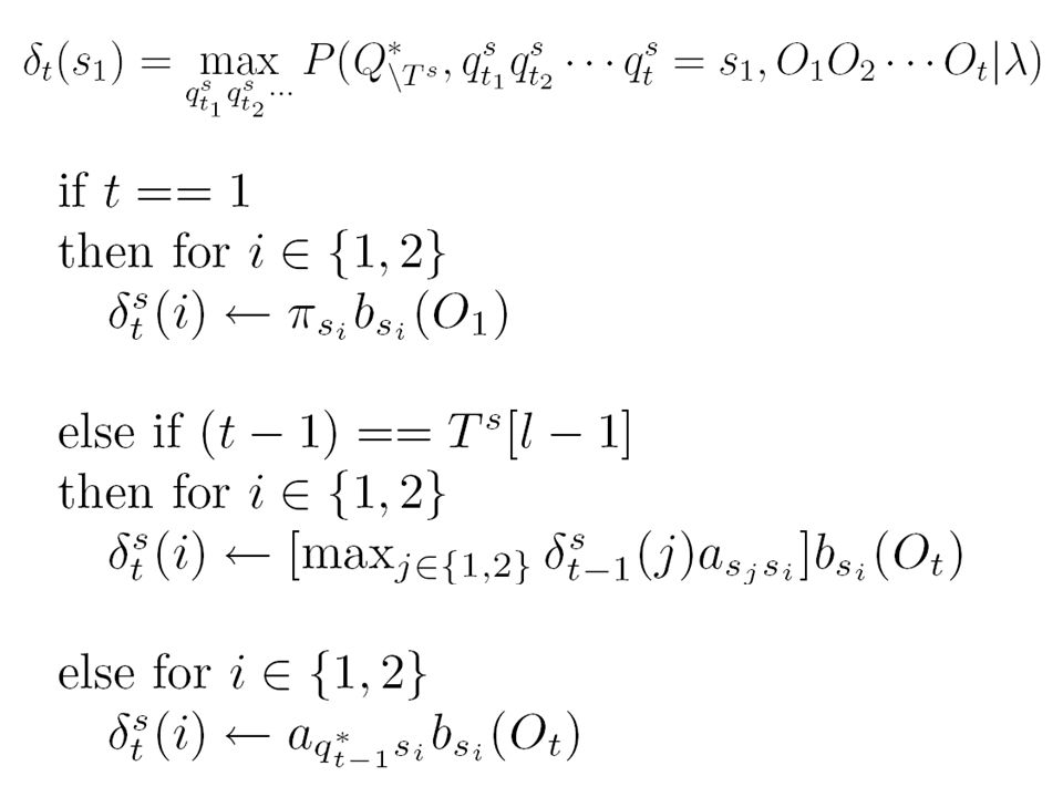
41. Constrained Viterbi Splitting state s to s 1,s 2. We calculate using a fast ‘constrained’ Viterbi algorithm over only those timesteps owned by s in Q *, and constraining them to belong to s 1 or s 2.

42. t δ  t (1)δ  t (2)δ  t (3) … δ  t (N) 1 2 3 4 5 6 7 8 9 The Viterbi path is denoted by Suppose we split state N into s 1,s 2

43. t δ  t (1)δ  t (2)δ  t (3) … δ  t (s 1 )δ  t (s 2 ) 1 2 3 4 5 6 7 8 9 ?? ?? ?? ?? The Viterbi path is denoted by Suppose we split state N into s 1,s 2

44. t δ  t (1)δ  t (2)δ  t (3) … δ  t (s 1 )δ  t (s 2 ) 1 2 3 4 5 6 7 8 9 The Viterbi path is denoted by Suppose we split state N into s 1,s 2

45. t δ  t (1)δ  t (2)δ  t (3) … δ  t (s 1 )δ  t (s 2 ) 1 2 3 4 5 6 7 8 9 The Viterbi path is denoted by Suppose we split state N into s 1,s 2

47. Iterate until convergence: Running time: O(|T s |n) per iteration When splitting state s, assumes rest of the HMM parameters ( \s ) and rest of the Viterbi path (Q * \Ts ) are both fixed OptimizeSplitParams I: Split-State Viterbi Training (SSVT)

48. Fast approximate BIC Compute once for base model: O(Tn 2 ) Update optimistically * for candidate model: O(|T s |) * first proposed in Stolcke and Omohundro, 1994

49. HMM Model Selection IV Initialize n 0 -state HMM randomly for n = n 0 … Nmax –Learn model parameters –for i = 1 … n Split state i, optimize by constrained EM Calculate approximate BIC score If best so far, store model –if larger model not chosen, stop

50. HMM Model Selection IV Initialize n 0 -state HMM randomly for n = n 0 … Nmax –Learn model parameters –for i = 1 … n Split state i, optimize by constrained EM Calculate approximate BIC score If best so far, store model –if larger model not chosen, stop Running time: O(Tn 2 ) per iteration of outer loop! O(Tn)

51. Algorithms SOFT: Baum-Welch / Constrained Baum-Welch HARD : Viterbi Training / Constrained Viterbi Training faster, coarser slower, more accurate

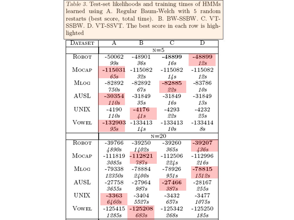
52. Results 1.Learning fixed-size models 2.Learning variable-sized models Baseline: Fixed-size HMM Baum-Welch with five restarts

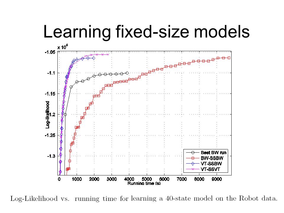
53. Learning fixed-size models

55. Fixed-size experiments table, continued

56. Learning fixed-size models

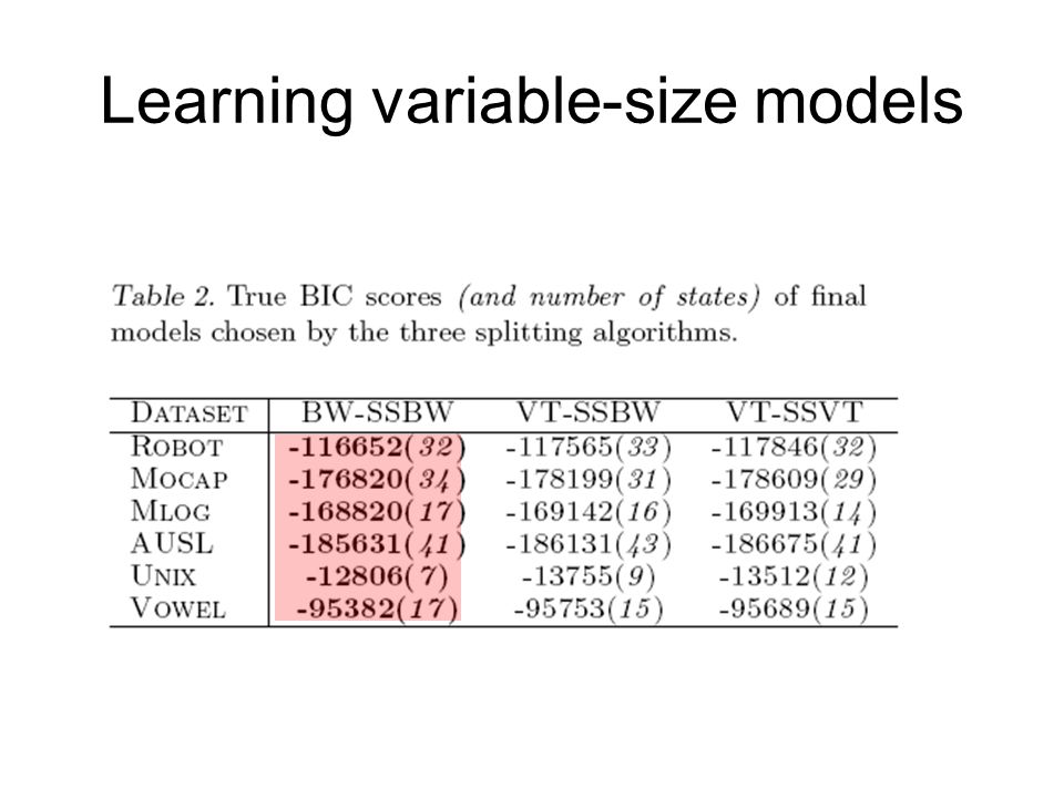
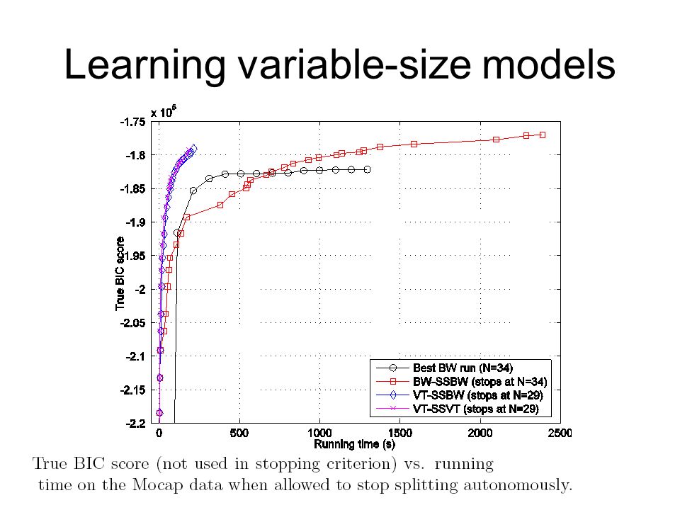
58. Learning variable-size models

63. Conclusion Pros: –Simple and efficient method for HMM model selection –Also learns better fixed-size models (Often faster than single run of Baum-Welch ) –Different variants suitable for different problems

64. Conclusion Cons: –Greedy heuristic: No performance guarantees –Binary splits also prone to local minima –Why binary splits? –Works less well on discrete-valued data Greater error from Viterbi path assumptions Pros: –Simple and efficient method for HMM model selection –Also learns better fixed-size models (Often faster than single run of Baum-Welch ) –Different variants suitable for different problems

65. Thank you

66. Appendix

67. Viterbi Algorithm

68. Constrained Vit.

69. EM for HMMs

71. More definitions

73. OptimizeSplitParams II: Constrained Baum-Welch Iterate until convergence:

74. Penalized BIC