1. MAE 552 Heuristic Optimization Instructor: John Eddy Lecture #18 3/6/02 Taguchi’s Orthogonal Arrays

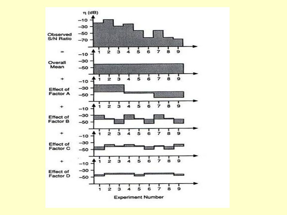
2. Additive Model

3. So from the previous result, we see that: m A3 = m + a 3 + some error term This is sensible enough, recall that our representation of a i was originally m Ai – m. So m A3 as we have derived it here, is an estimate of m + a 3 and thus our approach was in fact the use of an additive model.

4. Additive Model A note on the error term. We have shown that the error is actually the average of 3 error terms (one corresponding to each experiment). We typically treat each of the individual experiment error terms as having zero mean and some variance.

5. Additive Model Consider the expression to be the average variance of the 3 experiment error terms in our estimate of m A3. The error variance of our estimate of m A3 is then approximately (1/3). So this represents an approximate 3-fold reduction in error over a single experiment with factor A at level 3.

6. Additive Model Define Replication Number n r : –The replication number is the number of times a particular factor level is repeated in an orthogonal array. It can be shown that the error variance of the average effect of a factor level is smaller than the error variance of a single experiment by a factor equal to its n r.

7. Additive Model So, to obtain the same accuracy in our factor level averages using a one-at-a-time approach, we would have to conduct 3 experiments at each of the 3 levels of each factor. So in our example, if we choose temp to be our first factor to vary (holding all others constant), we would need to conduct:

8. Additive Model E(A 1, B 1, C 1, D 1 )3 times; E(A 2, B 1, C 1, D 1 )3 times and; E(A 3, B 1, C 1, D 1 )3 times; For a total of 9 experiments. We would then hold A constant at its best level and vary B for example. We would then need to conduct:

9. Additive Model E(A *, B 1, C 1, D 1 )0 times; E(A *, B 2, C 1, D 1 )3 times and; E(A *, B 3, C 1, D 1 )3 times; For a total of 6 additional experiments. We would then hold A and B constant at their best level and vary C for example. We would then need to conduct:

10. Additive Model E(A *, B *, C 1, D 1 )0 times; E(A *, B *, C 2, D 1 )3 times and; E(A *, B *, C 2, D 1 )3 times; For a total of 6 additional experiments. We would then hold A, B, and C constant at their best level and vary D. We would then need to conduct:

11. Additive Model E(A *, B *, C *, D 1 )0 times; E(A *, B *, C *, D 2 )3 times and; E(A *, B *, C *, D 3 )3 times; For a total of 6 additional experiments. The grand total is then 9+6+6+6 = 27 experiments.

12. Statistical Notes A statistical advantage of using Orthogonal arrays is that if the errors (e i ) are independent with zero mean and equal variance, then the estimated factor effects are mutually uncorrelated and we can determine the best level of each factor separately. You must conduct all experiments in the array or your approach will not be balanced, which is an essential property (we will lose orthogonality).

13. ANOVA We can get a general idea about the degree to which each factor effects the performance of our product/process by looking at the level means. This was suggested by our use of the factor effects in predicting observation values.

14. ANOVA An even better approach is to use a process called decomposition of variance, or commonly analysis of variance (ANOVA). ANOVA will also provide us with the means to estimate error variance for the factor effects and the variance of the error in a prediction.

15. ANOVA As a point of interest, we will discuss the analogy between ANOVA and Fourier analysis. Fourier analysis can be used to determine the relative strengths of the many harmonics that typically exist in an electrical signal. The large the amplitude of a harmonic, the more important it is to the overall signal.

16. ANOVA ANOVA is used to determine the relative importance of the various factors effecting a product or process. The analogy is as follows: –The obs. values are like the observed signal. –The sum-of-squared obs. values is like the power of the signal. –The overall mean is like the dc portion of the signal. –The factors are like harmonics –The harmonics of the signal are orthogonal as are the columns in our matrix.

18. ANOVA We’ll talk more about this analogy as we progress. For now, we need to define a few terms for use in our analysis of variance.

19. ANOVA Grand total sum-of-squares: –The sum the squares of all the observation values. (Is is the GTSOS that is analogous to the total power of our electrical signal.)

20. ANOVA Drawing our analogy to Fourier: –The sum of squares due to mean is analogous to the dc power of our signal and –The total sum of squares is analogous to the ac power of our signal.

21. ANOVA Grand total sum-of-squares: –The sum the squares of all the observation values. (Is is the GTSOS that is analogous to the total power of our electrical signal.)

22. ANOVA The GTSOS can be decomposed into 2 parts: –The sum of squares due to mean –The total sum of squares

23. ANOVA Drawing our analogy to Fourier: –The sum of squares due to mean is analogous to the dc power of our signal and –The total sum of squares is analogous to the ac power of our signal.

24. ANOVA Because m is the mean of the observation values, the total sum of squares can be written as: The derivation is shown on the following slide

25. ANOVA

26. So we can see from our previous results that the GTSOS is simply the sum of the SOSDTM and the TSOS as follows: In Fourier, the above result is analogous to the fact that the ac power of the signal is equal to the total power minus the dc power.

27. ANOVA What we need is the sum of squares due to each factor. These values will be a measure of the relative importance of the factors in changing the values of η. They are analogous to the relative strengths of our harmonics in our Fourier analysis.

28. ANOVA What we need is the sum of squares due to each factor. These values will be a measure of the relative importance of the factors in changing the values of η. They are analogous to the relative strengths of our harmonics in our Fourier analysis. They can be computed as follows:

29. ANOVA Sum of squares due to factor A Where (recall that) n r is the replication number and l is the number of levels.

30. ANOVA Lets go through and compute/look at these values for our example. 1 st notice that all of our replication numbers are 3. Our grand total sum of squares is:

31. ANOVA Our sum of squares due to the mean is: Our total sum of squares is:

32. ANOVA The sum of squares due to Factor A is:

33. ANOVA Using the same approach as for factor A, we can show that the remaining factor sum of squares are: For B:950(dB) 2 For C:350(dB) 2 For D: 50(dB) 2

34. ANOVA So from these calculations, we can determine exactly what percentage of the variation in η is due to each of the factors. This value is given by dividing the sum of squares for the factor by the total sum of squares. So we can say that: (2450/3800)*100 = 64.5% Of the variation in η is caused by factor A.

35. ANOVA Likewise: B:(950/3800)*100 = 25% C:(350/3800)*100 = 9.2% D:( 50/3800)*100 = 1.3% So we see that together, C and D account for only 10.5% of the variation in η.