1. Feedback Control Systems
Dr. Basil Hamed
Electrical & Computer Engineering
Islamic University of Gaza

2. STABILITY OF LINEAR FEEDBACK

3. PROBLEM DEFINITION
For people paralyzed from the neck down, the ability to drive themselves around in motorized wheelchairs is highly desirable.   A proposed system uses velocity sensors mounted in the headgear at 900 intervals, so that forward, left, right, or reverse directions can be commanded.   Output of the headgear sensor is proportional to the magnitude of the head movements.   The block diagram for this system is shown in figure 1.   Here, typical values for the time constants are 1 = 0.5 s, 3 = 1 s, and 4 = 1/4 s.

4. Using MATLAB do the following
1) Determine the limiting gain K = K1K2K3 for a stable system.
2) When the gain K is set equal to 1/3 of the limiting value, determine if the settling time to within 2% of the final value of the system is less than 4 s.
3) Determine the value of gain that results in a system with a settling time of 4 s.  Also, obtain the value of the roots of the characteristic equation when the settling time is equal to 4 s.

5. Block Diagram

6. Part 1)

7. Routh-Hurwitz Table
Routh-Hurwitz Table: s3          1          14         0 s2          7        8+8K       0 s1          A          0          0 s0        8+8K       0          0
A = -(8+8K-98) = K               7               7 For stability, A > 0, therefore 0 < K Therefore range for stability is given by:
0 < K < 11.25

8. Part 2) the closed-loop transfer function was found to be:
                  T(s) =                 8K                                              s3 + 7s2 + 14s K.
In calculating the settling time, we assume the validity of a second order approximation, allowing the use of the
dominant pole pair to find settling time as:
                  Ts =    4                              ζwn where ζwn = σd = -1 * real part of dominant poles. .
Poles are retrieved from function T(s) via the POLE command, producing a vector of s-plane coordinates. Since this system is third order, we expect this vector to contain 3 entries, the first for the real axis pole (to be far left from the dominant poles), and the remaining two as the dominant conjugate pole pair

9. Part 2)
K =
Open-loop system Transfer function: s^ s^ s + 1
Closed-loop system Transfer function:
s^ s^ s
P =
                      i           -     i
settling_time =  

10. Part 2)

11. Part 3)
For the system to be practical, a settling time of 4 seconds is required. Making use of the second order equation, settling time Ts = 4 / ζwn where ζwn = - real part of the dominant closed-loop pole pair, the settling time is calculated for each K value from 0.1 to the limiting gain or until one yielding a result of 4 seconds is found. The step response, transfer functions and the roots of the characteristic equation are displayed for this value of K.

12. Part 3) For K = 1.5 settling time is approximated as 4 seconds.
Open-loop transfer function with K = 1.5
Transfer function:                1.5
s^ s^ s + 1
Closed-loop transfer function with K = 1.5
Transfer function:                s^ s^ s + 2.5
Roots of the characteristic equation for K = 1.5
P =                              -1 +      i               -1  -      i
Settling time for K = 1.5
settling_time =   3.9999

13. Part 3)
Results show that K=1.5 yields an estimated settling time of seconds. From the step response, the simulation shows a settling time of 4.19 seconds which is close to the 4 seconds both approximated and required. Roots of the characteristic equation are also found by the program, with the three roots found being -5, -1+j1.73 and -1-j1.73.
The above step response also shows that this system has an overshoot of 14.8%, which is quite large. For a wheelchair application, where the comfort and safety of the user may be affected by such a large overshoot, further refinement of this system may be required

14. Animation

15. Problem 2

16. PROBLEM DEFINITION
The goal of vertical takeoff and landing (VTOL) aircraft is to achieve operation from relatively small airport and yet operate as normal aircraft in level flight. An aircraft taking off in a form similar to a missile (on end) is inherently unstable. A control system using adjustable jets can control the vehicle

17. Block Diagram

18. Use MATLAB
a) Find and plot closed loop poles in s-plane and discuss their location for K=100.
b) Determine the range of gain K for which the system is stable, marginally stable and unstable.
c) Determine and plot the roots of the characteristic equation for gain K obtained in part "b", which makes the system to be marginally stable and for selected gain K that makes the system unstable including poles locations from part "a" giving full comment.
d) Plot step responses of the system for K=100, selected system gain, which makes the system to be unstable and the obtained gain K in part "b" which makes the system to be marginally stable, giving comments on the obtained results.

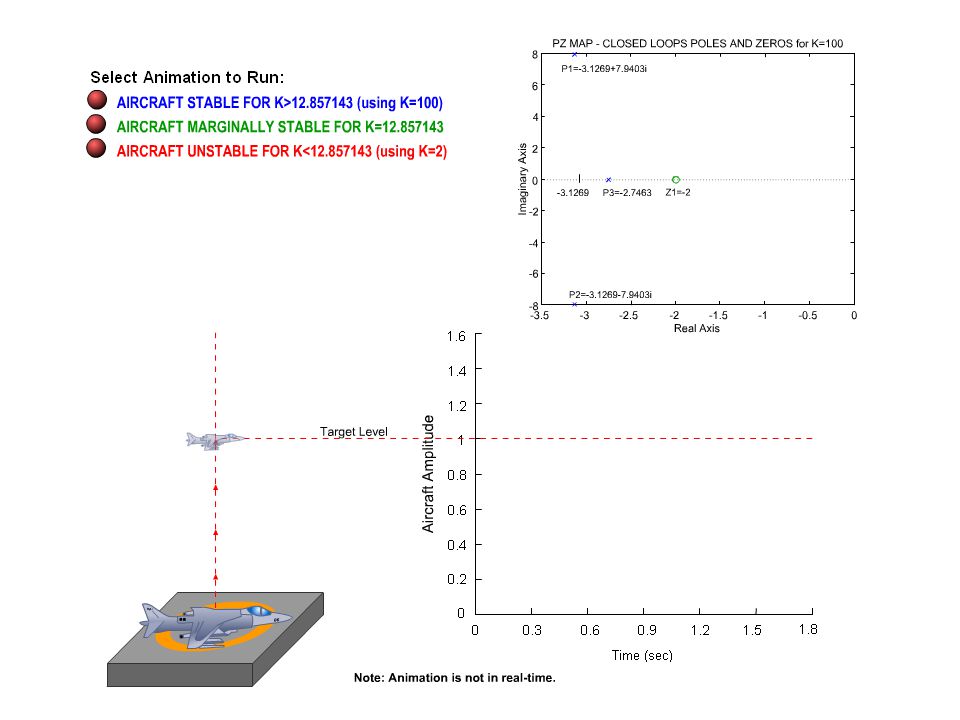
19. Part a) MATLAB results for K=100: P1= -3.1269+7.9403i ; zeros: z1= -2

20. Part a)
From closed loop poles and zeros plot above for system gain K=100 we can see that all (3) poles P1, P2  and P3 are located on the left side of s-plane (far away from the imaginary jw axis) soit is clear that system with K=100 is stable as any system pole is not placed on the right side of s-plane (rightaxis).

21. Part b) K<12.857143 - unstable K=12.875143 - marginally stable
K> stable

22. Part C)
The roots for selected K=2 (which make the system unstable) are:
P1=
P2= i
P3= i

23. Part C)

24. Part C) The roots for K=12.857143 (from part b) are: P1=-9
P2= i
P3= i
zeros: z1=-2

25. Part C)

26. Part D) Output step responses for K=100, K=12.8571 & K=2
Output step response of the aircraft control system

27. Output step response for K=100
From the above plot of output step response we can see the simulated system parameters: max OS%=57%, Tp=0.37sec, Ts=1.43sec and Tr=0.141.  Also taking in consideration the curve shape it can be concluded that the system is stable

28. Output step response for K=12.85714
From the above plot we can see system parameters such are max OS%, Tp, Tr and Ts, and also based on the curve shape, we can conclude that the system (aircraft) is marginally stable i.e. the system oscillates

29. Output step response for K=2
From the above plot it can be seen that the system (aircraft) is unstable, i.e. out of control as (see the curve shape) curve (aircraft) after reaching desired flight level of 1 is going up uncontrolled somewhere to infinity