1. Chapter 5: Calculating Earthquake Probabilities for the SFBR Mei Xue EQW March 16

2. Outline Introduction to Probability Calculations Calculating Probabilities Probability Models Used in the Calcuations Final calculation steps

3. Introduction to Probability Calculations

4. Earthquake probability is calculated over the time periods of 1-, 5-, 10-, 20-, 30- and 100-year-long intervals beginning in 2002 The input is a regional model of the long-term production rate of earthquakes in the SFBR (Chapter 4) The second part of the calculation sequence is where the time-dependent effects enter into the WG02 model

5. Introduction to Probability Calculations Review what time-dependent factors are believed to be important and introduce several models for quantifying their effects The models involve two inter- related areas: recurrence and interaction

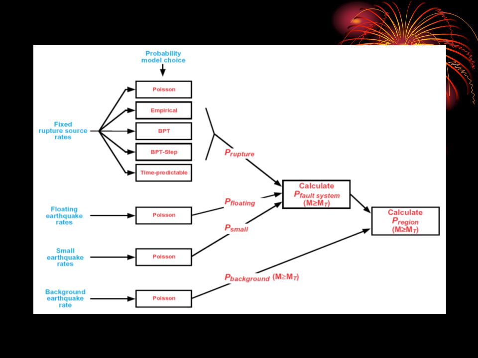
6. Introduction to Probability Calculations Express the likelihood of occurrence of one or more M  6.7 EQs in the SFBR in the time periods in five ways: The probability for each characterized large EQ rupture source (35) The probability that a particular fault segment will be ruptured by a large EQ (18) The probability that a large EQ will occur on any of the 7 characterized fault systems The probability of a background EQ (on faults in the SFBR, but not on one of the 7) The probability that a large EQ will occur somewhere in the region

7. Calculating Probabilities Primary input: the rupture source mean occurrence rate (Table 4.8) The probability rupture source, each fault, combined with background -> the probability for the region as a whole

8. Calculating Probabilities They model EQs that rupture a fault segment as a renewal process: independent Probability Models Poisson: the probability is constant in time and thus fully determined by the long-term rate of occurrence of the rupture source Empirical model: a variant of the Poisson, the recent regional rate of EQs Time-varying probability models: BPT, BPT- step (1906, 1989), and Time-predictable (1906), take into account information about the last EQ

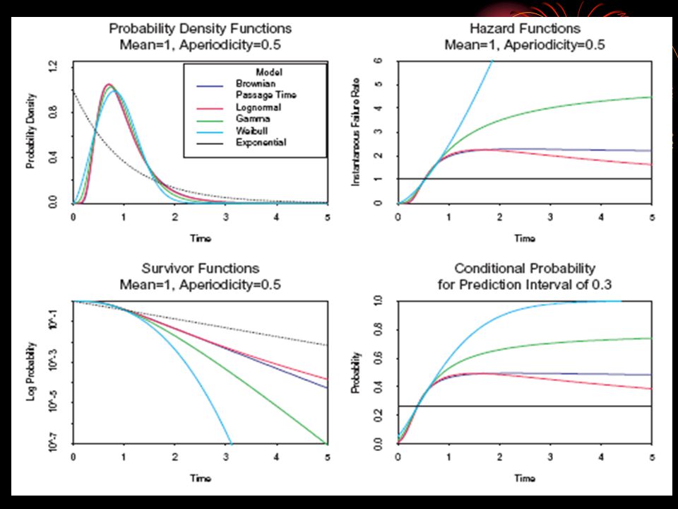
9. Calculating Probabilities Survivor function: gives the probability that at least time T will elapse between successive events Probability that one or more EQs will occur on a rupture source of interest during an interval of interest, conditional upon it not having occurred by T (year 2002) Conditional probability: gives the hazard function: gives the instantaneous rate of failure at time t conditional upon no event having occurred up to time t

10. Five Probability Models: 1 Poisoon Model - the mean rupture rate of each rupture source The hazard function is constant Fails to incorporate the most basic physics of the earthquake process: reloading Fails to account for stress shadow Reflects only the long-term rates Conservative estimate for faults that time- dependent models are either too poorly constrained or missing some critical physics (interaction)

12. Five Probability Models: 2 Empirical Model (t) – not stationary, estimated from the historical EQ record (M  3.0 since 1942 and M  5.5 since 1906) - the long term mean rate Complements the other models as M  5.5 is not used by other models Take into account the effect of the 1906 EQ stress shadow Specifies only time-dependence, preserving the magnitude distribution of the rupture sources

13. The shape of the magnitude distribution on each fault remains unchanged; the whole distribution moves up and down in time

15. Summary of rates and 30-year probabilities of EQs (M  6.7) in SFBR calculated with various models

16. Assumptions: 1.Fluctuations in the rate of M  3.0 and M  5.5 EQs reflect fluctuations in the probability of larger events 2.Fluctuations in rate on individual faults are correlated (though stress shadow is not homogeneous in space, affected seismicity on all magjor faults in the region) 3.The rate function  (t) can be sensibly extrapolated forward in time

17. Five Probability Models: 3 BPT Model μ – the mean recurrence interval, 1/ α – the aperiodicity, the variability of recurrence times, related to the variance  2, equals  /μ A Poisson process when α=1/sqrt(2)

18. 1.For smaller α, strongly peaked, remains close to zero longer 2. For larger α, “dead time” becomes shorter, increasingly Poisson-like

19. Estimates of aperiodicity α obtained by Ellsworth et al. (1999) for 37 EQ secquences (histogram) and the WG02 model (solid line)

20. Five Probability Models: 4 BPT-step Model A variation of the BPT model Account for the effects of stress changes caused by other earthquakes on the segment under consideration (1906, 1989) Interaction in the BPT-step model occurs through the state variable

21. 1.A decrease in the average stress on a segment lowers the probability of failure, while an increase in average stress causes an increase in probability 2.The effects are strongest when the segment is near failure

22. Assumptions: 1.The model represents the statistics of recurrence intervals for segment rupture 2.The time of the most recent event is known or constrained 3.The effects of interactions are properly characterized (BPT- step, 1906, 1989 San Andreas only)

23. Five Probability Models: 5 Time Predictable Model The next EQ will occur when tectonic loading restores the stress released in the most recent EQ Dividing the slip in the most recent EQ by the fault slip rate approximates the expected time to the next earthquake Only time of next EQ not size Only for the SAF fault

24. Five Probability Models: 5 Time Predictable Model Four extensions: 1.Model the SFBR as a network of faults 2.Strictly gives the probability that a rupture will start on a segment 3.Fault segments can rupture in more than one way 4.Use Monte Carlo sampling of the parent distributions to propagate uncertainty through the model

25. Five Probability Models: 5 Time Predictable Model Six-step calculation sequence: 1.Slip in the most recent event 2.Slip rate of the segment 3.Expected time of the next rupture of the segment 4.Probability of a rupture starting on the segment (4 segments, ignoring interaction, BPT model) – Epicentral probabilities 5.Convert epicentral probabilities into earthquake probabilities

26. Five Probability Models: 5 Time Predictable Model 6. Compute 30-year source probabilities

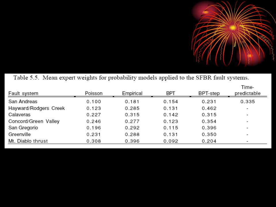
27. Final calculation steps Probabilities for fault segments and fault systems Probabilities for earthquakes in the background Weighting alternative probability models (VOTE) Probabilities for the SFBR model

31. Paper recommendataions Reasenberg, P.A., Hanks, T.C., and Bakun, W.H., 2003, An empirical model for earthquake probabilities in the San Francisco Bay region, California, 2002-2031, BSSA 93 (1): 1-13 FEB 2003 Shimazaki, K., and Nakata, T., Time-predictable recurrence model for large earthquakes: Geophysical Research Letters, v. 7, p. 279-282, 1980 Ellsworth, W.L., Matthews, M.V., Nadeau, R.M., Nishenko, S.P., Reasenberg, P.A., and Simpson, R.W., A physically- based earthquake recurrence model for estimation of long-term earthquake probabilities: USGS, OFR 99-522, 23 p., 1999 Cornell, C.A., and Winterstein, S.R., Temporal and magnitude dependence in earthquake recurrence models: BSSA, v. 78, no. 4, p. 1522-1537, 1988 Harris, R.A., and Simpson, R.W., Changes in static stress on Southern California faults after the 1992 Landers earthquake: Nature, v. 360, no. 6401, p. 251-254, 1992