Download presentation
Presentation is loading. Please wait.

1
Lectures on Center Vortices and Confinement Parma, Italia September 2005

2
Outline I.What is Confinement? II.Signals of the Confinement Phase III.Properties of the Confining Force IV.Confinement from Center Vortices V.Numerical Evidence VI.Connections to other ideas about confinement

3
Reviews: J.G., Prog. Nucl. Part. Phys. 51 (2003) 1; hep-lat/0301023 Michael Engelhardt, plenary talk at Lattice 2004, video and preprint available at http://lqcd.fnal.gov/lattice04
 1; hep-lat/ Michael Engelhardt, plenary talk at Lattice 2004, video and preprint available at")
4
Part I : What is Confinement? These lectures are mainly a review of the center vortex theory of confinement: a.Its motivation and formulation b.What we can learn from lattice strong-coupling expansions c.Evidence from lattice Monte-Carlo simulations d.Relations to other ideas (involving monopoles, or the Gribov Horizon) The numerical work is mostly for pure SU(2) Yang-Mills. Towards the end, I’ll discuss what happens when matter fields are added to the system. But to begin with: what are most people are trying to prove, when they talk about “proving” confinement? What are most of us are trying to explain, when we talk about “explaining” confinement?
 The numerical work is mostly for pure SU(2) Yang-Mills. Towards the end, I’ll discuss what happens when matter fields are added to the system. But to begin with: what are most people are trying to prove, when they talk about proving confinement. What are most of us are trying to explain, when we talk about explaining confinement .")
5
A. Historical: No free particles with 1/3, 2/3 electric charge. (Confinement?) From a modern point of view, this is kind of accidental. Suppose Nature has supplied us with a scalar field in the 3 representation of color SU(3), having otherwise vacuum quantum numbers. There would be free, fractionally charged particle states in the theory, although, if the scalars were very massive, the dynamics and spectrum of the theory wouldn’t otherwise be much different. B. Color Singlets: There exist no isolated, non-color-singlet particles in Nature. (Confinement?) While true, this definition is also a little problematic, because it also holds for gauge-Higgs theories in which the gauge group is completely broken spontaneously -- it can be interpreted as a color screening criterion.
 From a modern point of view, this is kind of accidental. Suppose Nature has supplied us with a scalar field in the 3 representation of color SU(3), having otherwise vacuum quantum numbers. There would be free, fractionally charged particle states in the theory, although, if the scalars were very massive, the dynamics and spectrum of the theory wouldn’t otherwise be much different. B. Color Singlets: There exist no isolated, non-color-singlet particles in Nature. (Confinement ) While true, this definition is also a little problematic, because it also holds for gauge-Higgs theories in which the gauge group is completely broken spontaneously -- it can be interpreted as a color screening criterion..")
6
Again consider adding a scalar field in the fundamental 3 representation of color SU(3) Two cases to consider: 2 > 0: unbroken SU(3). Color singlet spectrum, some additional quark-scalar bound states. External source shielded by bound state formation. 2 ¿ 0: spontaneous symmetry breaking. Still color singlet spectrum. External source shielded by condensate.

7
Non-abelian Gauss Law: rhs is the 0-component of a conserved current. Absence of a color E-field outside volume V means the non-abelian charge inside is zero. In the Higgs phase, the screening charge is supplied by the condensate. We get the same screening effect in the abelian Higgs model (an relativistic generalization of the Landau-Ginzburg superconductor), and even in an electrically charged plasma.
, and even in an electrically charged plasma..")
8
Inserting a charge +Q into an electrically charged plasma Charge is screened; but this is not what we mean by “confinement”.

9
The similarity - screening of heavy sources in both “broken” and “unbroken” gauge theories, is not a coincidence. Consider a gauge-Higgs lattice action Fradkin-Shenker Theorem There is no thermodynamic phase boundary in the G - H phase diagram, isolating the Higgs phase from a separate, confining phase. Consequence - Analytic free energy, no sudden qualitative change in the spectrum, e.g. from color singlets to non-singlets.

10
But : dynamics at H À 1 looks a lot like, e.g., Weinberg-Salam (without the photon), and much different from the dynamics of QCD. So lets focus on dynamics, rather than color singlets. What is special about the dynamics of QCD, as opposed to a Higgs theory? C. Regge Trajectories : In QCD, in a J vs. m 2 plot, mesons (and baryons) fall on linear, nearly parallel Regge trajectories. Why??
 fall on linear, nearly parallel Regge trajectories. Why .")
11
The “spinning stick” model: View a meson as a spinning line of length L=2R, with mass/length , and ends moving at the speed of light. Then, for the energy and the angular momentum Comparing the two expressions “Regge Slope”

12
From the data, ’ = 1/(2 = 0.9 Gev -2, which gives a string tension The model isn’t perfect (data has non-zero intercept, slightly different slopes). Allow for quantum fluctuations of the stick String Theory. How does a string-like picture come out of QCD? Flux tube formation!

13
So this is the interesting dynamics: Energy = L a linearly-rising potential between static sources (the “static quark potential”), and an infinite energy for infinite source separation. But is this what happens in real QCD?

14
String-Breaking and the Center of the Gauge Group In real QCD, with light fermions, as in the Fradkin-Shenker model, the linear potential does not extend indefinitely. For it is energetically favorable to pair-produce quarks, and break the flux tube (or QCD “string”).
..")
15
Then the static quark potential looks something like this At large distances, the color field of the static quarks are screened by the dynamical matter fields. Not so different from the Higgs physics.

16
If we want to explain the linear part of the potential, it is useful to work in a limit where the flux tube never breaks (“permanent confinement”), screening is suppressed, and the potential rises linearly without leveling out. In this limit, for any finite gauge group and set of matter fields, we now take note of an important fact: Permanent confinement exists only if: 1.the unbroken gauge group has a non- trivial center subgroup, and 2.all matter fields transform as singlets wrt that center subgroup. There are no known exceptions (G(2) is an example, not an exception). This fact provides us with an important clue about the nature of confinement.
 is an example, not an exception). This fact provides us with an important clue about the nature of confinement..")
17
A little group theory: The center of a Lie Group consists of those group elements which commute with all elements of the group. For an SU(N) gauge theory, this is the set of all group elements proportional to the identity: which form the discrete abelian subgroup Z N of SU(N). There are an infinite no. of representations of SU(N), but only a finite number of representations of Z N. Every representation of SU(N) falls into one of N subsets (known as “class” or “N-ality”), depending on the representation of the Z N subgroup.
 gauge theory, this is the set of all group elements proportional to the identity: which form the discrete abelian subgroup Z N of SU(N). There are an infinite no. of representations of SU(N), but only a finite number of representations of Z N. Every representation of SU(N) falls into one of N subsets (known as class or N-ality ), depending on the representation of the Z N subgroup..")
18
l N-ality is given by the number of boxes in the Young tableau, mod N. Multiplication by a center element z n, in a representation of N-ality k, corresponds to multiplication by a factor of l N-ality = 0 representations (e.g. the adjoint representation) are special, in that all center elements map onto the identity. l Particles of N-ality = 0 cannot bind to a particle of N-ality 0 to form a singlet. l Consequence: Particles in N-ality = 0 representations can never break the string connecting two N-ality 0 sources.
 are special, in that all center elements map onto the identity. l Particles of N-ality = 0 cannot bind to a particle of N-ality 0 to form a singlet. l Consequence: Particles in N-ality = 0 representations can never break the string connecting two N-ality 0 sources..")
19
So the limit in which the linear potential (if it exists) rises indefinitely, is the limit in which l for QCD (or any SU(N) theory): take the masses of the quarks to infinity. l for G(2), introduce a Higgs and break the gauge group to SU(3), taking the mass of the massive gluons to infinity. Our goal (and the strategy of most efforts in this field) is to try to understand the linear potential in limit that it goes on forever. Once we understand confinement in this limit, we can take the masses of quarks (or broken generator gluons) to be finite, and see how the picture changes.
, introduce a Higgs and break the gauge group to SU(3), taking the mass of the massive gluons to infinity. Our goal (and the strategy of most efforts in this field) is to try to understand the linear potential in limit that it goes on forever. Once we understand confinement in this limit, we can take the masses of quarks (or broken generator gluons) to be finite, and see how the picture changes..")
20
Part II : Signals of Confinement A. The Wilson Loop The Wilson loop has a dual role: l rectangular timelike loops are related to the interaction potential of static, external sources, l spacelike loops are probes of gauge-field fluctuations in the vacuum state, independent of external sources Of course, spacelike and timelike loops are not intrinsically different, but related to one another by Lorentz (or, Euclidean rotation) invariance. It means that the interaction energy between static sources is related to vacuum fluctuations in the absence of external sources. Lets start with the relation of timelike loops to the static quark potential.
 invariance. It means that the interaction energy between static sources is related to vacuum fluctuations in the absence of external sources. Lets start with the relation of timelike loops to the static quark potential..")
21
Start with an SU(N) lattice gauge field, and a single quark field in color group representation r. The quark field is so massive that all quarks are static, and string-breaking effects can be ignored. Let Q be an operator which creates a color-singlet quark-antiquark state, with separation R

22
By the usual rules For m q very large, this is evaluated by bringing terms down from the action, and we find

23
Where r (g) is the group character (trace) of group element g in representation r, U(R,T) is the holonomy - ordered product of link variables around the loop - and W r (R,T) is the VEV “Holonomy” is just a Wilson loop, before taking the trace. In the continuum, the holonomy U(C) is
 is.")
24
Digression on Character Expansions A class function F[g] is a function defined on the group manifold, with the property that for any two group elements g and h A class function can always be expanded in terms of group characters, where the sum is over representations r, and the group character is the trace of group element g in representation r. A Fourier series expansion is an example of a character expansion; in this case the group is U(1), the sum runs over positive and negative integers, and n [e i ] = e in
![Digression on Character Expansions A class function F[g] is a function defined on the group manifold, with the property that for any two group elements g and h A class function can always be expanded in terms of group characters, where the sum is over representations r, and the group character is the trace of group element g in representation r.](http://images.slideplayer.com/16/5113937/slides/slide_24.jpg "A Fourier series expansion is an example of a character expansion; in this case the group is U(1), the sum runs over positive and negative integers, and n [e i ] = e in .")
25
So now we have The minimal energy is singled out in the T ! 1 limit. The R-dependent part of the potential is obtained from and this is what we refer to as the static quark potential in group representation r. The confinement problem is to show that at large R, for N-ality 0 representations, or more generally

26
an asymptotic, area-law falloff B. The Polyakov Line In an SU(N) gauge theory with only N-ality=0 matter fields there is, beyond the SU(N) gauge symmetry, an additional global Z n symmetry on a finite periodic lattice:
 gauge theory with only N-ality=0 matter fields there is, beyond the SU(N) gauge symmetry, an additional global Z n symmetry on a finite periodic lattice:.")
27
This transformation does not change plaquettes or Wilson loops. But there are certain gauge-invariant observables which are affected.

28
Consider a Wilson line which winds once around the lattice in the periodic time direction This is known as a Polyakov Loop. Under a center transformation U 0 (x,t 0 ) z U 0 (x,t 0 ), we find This global symmetry can be realized on the lattice in one of two ways: This has a lot to do with confinement, because…
 z U 0 (x,t 0 ), we find This global symmetry can be realized on the lattice in one of two ways: This has a lot to do with confinement, because….")
29
a Polyakov line can be thought of as the world-line of a massive static quark at fixed spatial position x, propagating through the periodic time direction. Then where F q is the quark free energy. In the confinement phase, the free energy is infinite, but finite in a non-confined phase. So unbroken Z N symmetry = confinement phase Actually the transformation U 0 (x,t 0 ) z U 0 (x,t 0 ) can be generalized; it is a special example of a singular gauge transformation. Consider Periodic only up to a center transformation
 z U 0 (x,t 0 ) can be generalized; it is a special example of a singular gauge transformation. Consider Periodic only up to a center transformation.")
30
This again transforms Polyakov lines P(x) z P(x), but plaquettes and ordinary Wilson loops are not affected. In the continuum, it amounts to transforming the gauge field by the usual formula Except, at t=L t, we drop the second term (which would be a delta-function). Because of that, a “singular gauge transformation” is not a true gauge transformation.
. Because of that, a singular gauge transformation is not a true gauge transformation..")
31
C. The ‘t Hooft Loop Instead of gauge transformations which are discontinuous on loops which wind around the periodic lattice, which could also consider transformations which are discontinuous on other sets of loops. In fact there is a familiar example in classical electrodynamics: the exterior field of a solenoid is the result of a singular gauge transformation applied to A=0 ! So lets start with electrodynamics. The Wilson loop holonomy U(1) is C is spacelike, B is the magnetic flux through the loop.
 is C is spacelike, B is the magnetic flux through the loop..")
32
We can have B non-zero, yet B=0 along C. E.g., the vector potential exterior to a solenoid of radius R, oriented along the z-axis which is obtained from a singular gauge transformation of A=0, with Note the discontinuity We drop the delta-function that would arise in A if this were a true gauge transformation.

33
It’s the exp[i B ] discontinuity at =0,2 which is essential. Consider a loop winding n times around the z-axis: linking number = n. Any singular gauge transformation, with the same discontinuity, applied to any vector potential A, would give The concept of linking: loop C (B=0) Solenoid (B 0) line of discontinuity in g( )
![It’s the exp[i B ] discontinuity at =0,2 which is essential.](http://images.slideplayer.com/16/5113937/slides/slide_33.jpg "Consider a loop winding n times around the z-axis: linking number = n. Any singular gauge transformation, with the same discontinuity, applied to any vector potential A, would give The concept of linking: loop C (B=0) Solenoid (B 0) line of discontinuity in g( ).")
34
Loops link to points (D=2), other loops (D=3), surfaces (D=4). In our example, the solenoid is a surface in the z-t plane in D=4 dimensions, and the gauge discontinuity lies on a 3-volume at y=0, x>0.

35
Summarize: the singular gauge transformation creates a surface of magnetic flux in the z-t plane, and any Wilson loop holonomy which is topologically linked to this surface gets multiplied by a factor of exp[i B ] U(1). Generalize to SU(N) We consider: l g(x) discontinuous on a Dirac 3-volume V 3 l g(x) creates magnetic flux only on the boundary S of the 3-volume Let C be a loop which is topologically linked to S, parametrized by with
![Summarize: the singular gauge transformation creates a surface of magnetic flux in the z-t plane, and any Wilson loop holonomy which is topologically linked to this surface gets multiplied by a factor of exp[i B ] U(1).](http://images.slideplayer.com/16/5113937/slides/slide_35.jpg "Generalize to SU(N) We consider: l g(x) discontinuous on a Dirac 3-volume V 3 l g(x) creates magnetic flux only on the boundary S of the 3-volume Let C be a loop which is topologically linked to S, parametrized by with.")
36
What kind of discontinuity can g(x) have? Suppose g(x(1)) = h g(x(0)) where h is any SU(N) group element. In general this introduces a field strength throughout V 3. But, as with center transformations in a periodic volume, we are looking for a discontinuity which changes the loop holonomy U[C], without changing the action in the neighborhood of C. This is accomplished by so that If this is true for any loop linked to S, no matter how small, then it means that the singular transformation has created a surface of infinite field strength just on S. Its called a thin center vortex. As in QED, the singular region can be smeared out in a region of finite thickness, a kind of solenoid sweeping out S. This is a thick center vortex.
) = h g(x(0)) where h is any SU(N) group element. In general this introduces a field strength throughout V 3. But, as with center transformations in a periodic volume, we are looking for a discontinuity which changes the loop holonomy U[C], without changing the action in the neighborhood of C. This is accomplished by so that If this is true for any loop linked to S, no matter how small, then it means that the singular transformation has created a surface of infinite field strength just on S. Its called a thin center vortex. As in QED, the singular region can be smeared out in a region of finite thickness, a kind of solenoid sweeping out S. This is a thick center vortex..")
37
Creating a thin vortex on the lattice: On every x-y plane of the lattice, set The thin vortex is a stack of plaquettes at x 0,y 0 at all z,t. This is a surface. Note that if the discontinuity were not a center element, then the action would be affected at all plaquettes in the Dirac volume.

38
Go to the Hamiltonian formulation, and let B[C] be an operator which creates a thin center vortex at fixed time t along curve C. This means that B[C] performs a singular gauge transformation on gauge fields at time t. It follow that along any loop C’ linked to C in D=3 dimensions, Using only this relation, ‘t Hooft argued that l only area-law or perimeter-law falloff for, is possible, l in the absence of massless excitations, it is impossible to have So, perimeter law for B[C] implies area-law falloff for U[C] (i.e. confinement).
![Go to the Hamiltonian formulation, and let B[C] be an operator which creates a thin center vortex at fixed time t along curve C.](http://images.slideplayer.com/16/5113937/slides/slide_38.jpg "This means that B[C] performs a singular gauge transformation on gauge fields at time t. It follow that along any loop C’ linked to C in D=3 dimensions, Using only this relation, ‘t Hooft argued that l only area-law or perimeter-law falloff for, is possible, l in the absence of massless excitations, it is impossible to have So, perimeter law for B[C] implies area-law falloff for U[C] (i.e. confinement)..")
39
C. The Vortex Free Energy (Introduced by ‘t Hooft, first simulations by Kovacs and Tomboulis, much further work by de Forcrand and von Smekal) Consider a finite 2D lattice. Usually we impose periodic boundary conditions Lets modify this by the following condition: This boundary condition can be absorbed into a change in the coupling ! z at the single plaquette P’ that contains U y (L,y 0 ), i.e
 Consider a finite 2D lattice. Usually we impose periodic boundary conditions Lets modify this by the following condition: This boundary condition can be absorbed into a change in the coupling . z at the single plaquette P’ that contains U y (L,y 0 ), i.e.")
40
This is an example of twisted boundary conditions. It is impossible, with this choice, to pick the link variables such that the action vanishes. The twisted b.c. introduces a Dirac string, starting at (L,y 0 ). But it has to end somewhere; at the end is a center vortex. This is the rough argument; see ‘t Hooft for more rigor in showing that t.b.c. introduce a unit of center flux.
. But it has to end somewhere; at the end is a center vortex. This is the rough argument; see ‘t Hooft for more rigor in showing that t.b.c. introduce a unit of center flux..")
41
Generalization to higher dimensions is straighforward: A single link in D=2 becomes a line of links in D=3, and surface of links in D=4 For simplicity, consider SU(2), and z = -1 for twisted boundary conditions. We define Z + as the lattice partition function with ordinary boundary conditions, and Z - as the partition function with twisted boundary conditions. The magnetic free energy of a Z 2 vortex is then given by The “electric” free energy is defined by a Z 2 Fourier transform

42
Then let C be a rectangular loop of area A[C]. The following inequality was proved by Tomboulis and Yaffe So, if the vortex free energy falls off wrt cross-sectional area L x L y like then this is a sufficient condition for confinement, because it implies an area law bound for Wilson loops. Numerical investigations of these quantities were begun by Kovacs and Tomboulis, and carried on in much more detail by de Forcrand and von Smekal.
![Then let C be a rectangular loop of area A[C].](http://images.slideplayer.com/16/5113937/slides/slide_42.jpg "The following inequality was proved by Tomboulis and Yaffe So, if the vortex free energy falls off wrt cross-sectional area L x L y like then this is a sufficient condition for confinement, because it implies an area law bound for Wilson loops. Numerical investigations of these quantities were begun by Kovacs and Tomboulis, and carried on in much more detail by de Forcrand and von Smekal..")
43
This is the first numerical computation of Z - /Z + Consistent with vortex free energy going rapidly to zero at large lattice volume. Kovacs and Tomboulis.

44
To Repeat The existence of a non-zero asymptotic string tension requires that 1.The gauge group has a non-trivial center 2.All matter fields transform in N-ality=0 representations In that case, the action is invariant under global center transformations. All of the signals we’ve seen for non-vanishing asymptotic string tension: a)area law for Wilson loops b)vanishing Polyakov lines c)perimeter-law ‘t Hooft loops d)area-law falloff for the vortex free energy can only be satisfied if global center symmetry exists. This motivates the idea that vacuum fluctuations responsible for the asymptotic string tension must be, in some way, connected with center symmetry.
area law for Wilson loops b)vanishing Polyakov lines c)perimeter-law ‘t Hooft loops d)area-law falloff for the vortex free energy can only be satisfied if global center symmetry exists. This motivates the idea that vacuum fluctuations responsible for the asymptotic string tension must be, in some way, connected with center symmetry..")
45
Part III : Properties of the Confining Force l Asymptotic Linearity of the Static Potential l Casimir Scaling l N-ality dependence l String Behavior: Roughening and the Luscher term Asymptotic Linearity Theorem: the force between a static quark and antiquark is everywhere attractive but cannot increase with distance; i.e. The potential is convex, and can rise no faster than linear. (Bachas)
.")
46
Since We can compute the static potential from There are techniques for greatly increasing convergence to the large-T limit by “smearing” the spacelike links.

47
Here is a typical numerical result for the static potential Necco and Sommer

48
Casimir Scaling This is the idea that there is some intermediate range of distances where the string tension between a quark in group representation r, and its antiquark, is approx. proportional to the quadratic Casimir C r of the representation. Why? - Two arguments: large-N limit, and dimensional reduction. Large-N: Group character r (g) = trace of g in representation r has the property n+m ¿ N is the smallest integer such that the irreducible representation r is obtained from the reduction of a product of n defining (``quark'') representations, and m conjugate (``antiquark'') representations. Ambjorn & Olesen, Faber et al.
 = trace of g in representation r has the property n+m ¿ N is the smallest integer such that the irreducible representation r is obtained from the reduction of a product of n defining (``quark ) representations, and m conjugate (``antiquark ) representations. Ambjorn & Olesen, Faber et al..")
49
Large-N also has the property of factorization: if A and B are two gauge- Invariant operators, then Put these facts together: It follows that which is precisely Casimir scaling in this large-N limit.

50
Its interesting to see how this goes in lattice strong-coupling expansions. The adjoint representation is n=m=1, and we find, for a square LxL loop in SU(N) where the second term comes from a “double layer” of plaquettes in the minimal area, and the second comes from the “tube” diagram
 where the second term comes from a double layer of plaquettes in the minimal area, and the second comes from the tube diagram.")
51
At large-N the first term / N 2 dominates initially, but eventually, for The perimeter term takes over, and the adjoint string tension drops to zero (n-ality dependence). The second argument for Casimir scaling was: Dimensional Reduction (J.G., Olesen) At strong-coupling, confinement in D=4 looks the same as D=2. But in D=2, its easy to show that the confining potential at weak coupling comes from one-gluon exchange, and this leads to Casimir scaling. So is confinement at weak-coupling in D=4 something like confinement at weak-coupling in D=2?
 At strong-coupling, confinement in D=4 looks the same as D=2. But in D=2, its easy to show that the confining potential at weak coupling comes from one-gluon exchange, and this leads to Casimir scaling. So is confinement at weak-coupling in D=4 something like confinement at weak-coupling in D=2 .")
52
Argument: consider a spacelike Wilson loop In temporal gauge, R[A] is gauge-invariant, so we consider an expansion For small amplitude, long-wavelength configurations, perhaps only the first term dominates, in which case
![Argument: consider a spacelike Wilson loop In temporal gauge, R[A] is gauge-invariant, so we consider an expansion For small amplitude, long-wavelength configurations, perhaps only the first term dominates, in which case](http://images.slideplayer.com/16/5113937/slides/slide_52.jpg "Argument: consider a spacelike Wilson loop In temporal gauge, R[A] is gauge-invariant, so we consider an expansion For small amplitude, long-wavelength configurations, perhaps only the first term dominates, in which case")
53
Dimensional reduce one more time, to get Since we have Casimir scaling in D=2, we should then get Casimir scaling in D=4. Numerically, this works pretty well. Here is some data for SU(3): (Bali) Solid lines are a fit to the fundamental data, Multiplied by the Casimir ratio C r /C F
: (Bali) Solid lines are a fit to the fundamental data, Multiplied by the Casimir ratio C r /C F.")
54
N-ality Dependence Consider a quark-antiquark pair in representation r, with N-ality k r. Gluons can bind to the quark and antiquark, and reduce the color charge to the lowest-dimensional representation with the same N-ality k r. It follows that the after screening by gluons - i.e. asymptotically, string tension depends only on N-ality, String tensions of the lowest-dimensional representation of N-ality k are often called “k-string tensions”. Two proposals for SU(N) gauge theories: “Casimir scaling” (a slight misnomer!) Sine-law scaling Either way, (k) / k for k ¿ N.
 gauge theories: Casimir scaling (a slight misnomer!) Sine-law scaling Either way, (k) / k for k ¿ N..")
55
For our purposes, the crucial point is not Casimir vs Sine Law, but rather the simple fact that asymptotic string tension depends only on the N-ality of the representation. An important example: the adjoint representation, which has k=0. We get string-breaking, and a flat static (adjoint) quark potential, when where m GL is the mass of the adjoint quark-gluon bound state. de Forcrand & Kratochvila
 quark potential, when where m GL is the mass of the adjoint quark-gluon bound state. de Forcrand & Kratochvila.")
56
String Behavior (Luscher) If the QCD flux tube resembles a Nambu string, then transverse fluctuations of the string induce a universal (coupling, scale) independent 1/R modificiation to the linear potential According to the string calculation, the cross-sectional area of the flux tube should also grow logarithmically with R. Both of these effects have been observed in numerical simulations. (Luscher & Weisz, Kuti et al.) the “Luscher term”
 the Luscher term .")
57
Part IV: Confinement from Center Vortices The motivations we’ve already seen: l Confinement - non-vanishing asymptotic string tension - is associated with the unbroken realization of a global center symmetry. The asymptotic string tension depends only on N-ality. In particular, whatever vacuum fluctuations cause F 0 should not also force A 0. l Two of the order parameters for confinement - the ‘t Hooft loop B[C] and the vortex free energy, are explicitly associated with the center vortex creation, while the non-zero value of the Polyakov line is a signal of spontaneous center symmetry breaking. What can we learn from strong-coupling expansions, where confinement can be derived analytically?

58
Lets consider SU(2) lattice gauge theory at strong couplings, and U[C] is an SU(2) holonomy around loop C. Suppose C is very large, and we subdivide the minimal area into a set of sub-areas bounded by {U(C i )} as shown Do the individual holonomies C i fluctuate independently, if all loops are very large, or are they correlated somehow?
![Lets consider SU(2) lattice gauge theory at strong couplings, and U[C] is an SU(2) holonomy around loop C.](http://images.slideplayer.com/16/5113937/slides/slide_58.jpg "Suppose C is very large, and we subdivide the minimal area into a set of sub-areas bounded by {U(C i )} as shown Do the individual holonomies C i fluctuate independently, if all loops are very large, or are they correlated somehow .")
59
In general - observables a,b,c… are uncorrelated iff = …. So lets find out if where F[g] is any class (gauge inv) function with s dg F[g] =0. Such functions can be expanded in group characters If we evaluate the VEVs in D=2 dimensions, the equality is satisfied (and dominated by the lowest dimensional group representation) This works because.
 function with s dg F[g] =0. Such functions can be expanded in group characters If we evaluate the VEVs in D=2 dimensions, the equality is satisfied (and dominated by the lowest dimensional group representation) This works because..")
60
But for D>2, the N-ality=0 group characters have an asymptotic perimeter law falloff, and the lowest dimensional of these (j=1) dominates the VEVs. At strong coupling, we find Because CONCLUSION: At D>2 the U(C i ) do not fluctuate independently. But how does the area law arise, for j=half-integer Wilson loops? Extract a center element from the holonomies And ask if these fluctuate independently.
 do not fluctuate independently. But how does the area law arise, for j=half-integer Wilson loops. Extract a center element from the holonomies And ask if these fluctuate independently..")
61
i.e., does It does! Confining disorder (for D>2) is center disorder, at least at strong couplings. It is natural to suspect that the source of this disorder is the center vortices, which affect loop holonomies only by a factor of a center element. Its therefore interesting that thin center vortices are saddlepoints of the strong-coupling effective action.

62
Start with the strong-coupling Wilson action on a “fine” lattice of lattice spacing a and do a “blocking” transformation to arrive at an effective action on a lattice with spacing a’=La U’-link

63
The blocking transformation can be carried out analytically, and the result is (Faber et al.) For simplicity, truncate to the leading one-plaquette terms…
 For simplicity, truncate to the leading one-plaquette terms…")
64
with Question: Does this action have a local minimum, other than vacuum (U=I)? Answer: Yes, for c 1 À c 0 any center configuration, gauge-equivalent to is a saddlepoint (local minimum) of the effective action, where is a center element.
 of the effective action, where is a center element..")
65
Proof: Consider small fluctuations of link variables around center elements And denote the product of V links around a plaquette as V P Then the effective action, to O(F P 2 ) is We see by inspection that for c 1 À c 0, the action has a local minimum at F P =0. QED.

66
Now we move away from strong coupling, and suppose that vacuum configurations in SU(N) gauge theory can be decomposed into a relatively smooth confining background, and high-frequency fluctuations around that background An important hint about is N-ality dependence. An N-ality = 0 Wilson loop should have no area law falloff; i.e. should be not depend much on. Suppose its not affected at all. Then, writing holonomies Confining background fluctuations

67
it means that for N-ality=0 But this can only be true if (up to a gauge transformation) Link variables which give center element holonomies are gauge-equivalent To the link variables of a Z N lattice gauge theory whose excitations consist only of center vortices.
 Link variables which give center element holonomies are gauge-equivalent To the link variables of a Z N lattice gauge theory whose excitations consist only of center vortices.")
68
The Center Vortex Confinement Mechanism (finally!) We assume that variables can be expressed such that 1.large holonomies u[C] and Z[C] are only weakly correlated 2. for any two large non-overlapping loops as we found to be true in strong-coupling lattice gauge theory. This is enough to give us confinement!
![The Center Vortex Confinement Mechanism (finally!) We assume that variables can be expressed such that 1.large holonomies u[C] and Z[C] are only weakly correlated 2.](http://images.slideplayer.com/16/5113937/slides/slide_68.jpg "for any two large non-overlapping loops as we found to be true in strong-coupling lattice gauge theory. This is enough to give us confinement!.")
69
Here’s how: Consider for simplicity a large rectangular Wilson loop C of area A, in group representation r of N-ality k. We have, by assumption Now subdivide the area A into square LxL subareas bounded by loops {C i }. where An area law which depends only on N-ality

70
How big should we make these LxL subareas? (It doesn’t matter, as long as the Z(C k ) are uncorrelated.) Very simplest case: LxL is 1x1. This means that the probability f for a given plaquette p to have z(p) = -1 is uncorrelated with the values of z(p’) on other plaquettes p’ in the same plane.
 are uncorrelated.) Very simplest case: LxL is 1x1. This means that the probability f for a given plaquette p to have z(p) = -1 is uncorrelated with the values of z(p’) on other plaquettes p’ in the same plane..")
71
Lets run through the argument again. The decomposition Dirac line gives us a confining background of thin center vortices (the z (x)), With non-confining fluctuations gug -1 around that background.
), With non-confining fluctuations gug -1 around that background..")
72
Wilson loop W[C] is multiplied by a factor of z for each vortex piercing the minimal area.
![Wilson loop W[C] is multiplied by a factor of z for each vortex piercing the minimal area.](http://images.slideplayer.com/16/5113937/slides/slide_72.jpg "Wilson loop W[C] is multiplied by a factor of z for each vortex piercing the minimal area.")
73
Then and and assume that 1.Piercings are uncorrelated; 2.Fluctuations u[C] are uncorrelated with Z[C] for large loops Again define f = prob. that a vortex pierces any given plaquette = prob. that z(p) = -1 Denote
![Then and and assume that 1.Piercings are uncorrelated; 2.Fluctuations u[C] are uncorrelated with Z[C] for large loops Again define f = prob.](http://images.slideplayer.com/16/5113937/slides/slide_73.jpg "that a vortex pierces any given plaquette = prob. that z(p) = -1 Denote.")
74
Then String tensions are and depend only on N-ality.

75
Part V: Numerical Evidence The vortex mechanism is probably the simplest route to confinement, and well motivated by local gauge-invariant order parameters for confinement (‘t Hooft loop, Polyakov loop, vortex free energy), and by the known facts about N-ality dependence. But is it right? To find out, we turn to lattice Monte Carlo simulations. The first problem is to figure out how to spot thick center vortices in a list of what looks like random numbers - i.e. the lattice link variables.

76
Finding Center Vortices in Thermalized Lattices An “adjoint gauge” is a gauge which completely fixes link variables U A in the adjoint representation, leaving a residual Z N gauge symmetry. An example is the adjoint Landau gauge, which maximizes This gauge is also known as direct maximal center gauge. In an adjoint gauge, we factor each link variable into a center and coset part where Z (x) is the center element closest to U (x) on the Lie group manifold. E.g., for SU(2): Z (x) = signTr[U (x)].
 is the center element closest to U (x) on the Lie group manifold. E.g., for SU(2): Z (x) = signTr[U (x)]..")
77
Center Projection is the replacement of link variables U in an adjoint gauge by their closest center elements, i.e. which maps the SU(N) configuration into a Z N configuration. Plaquettes Z(p) 1 on the projected lattice are known as P-plaquettes, and together they form thin center vortices known as P-vortices. The claim is that this procedure locates center vortices on the unprojected lattice. The idea is that P-vortices lie somewhere in the middle of the “thick” center vortices on the uprojected lattice.
 configuration into a Z N configuration. Plaquettes Z(p) 1 on the projected lattice are known as P-plaquettes, and together they form thin center vortices known as P-vortices. The claim is that this procedure locates center vortices on the unprojected lattice. The idea is that P-vortices lie somewhere in the middle of the thick center vortices on the uprojected lattice..")
78
Motivation Suppose we have some lattice configuration U, and insert “by hand” a thin center vortex, via a singular gauge transformation, somewhere on the lattice. Will this center vortex be among the set of vortices identified by the center projection procedure? The answer is yes. Let U’ be the lattice with the inserted vortex. In the adjoint representation, the corresponding U A and U’ A are gauge-equivalent. Then in adjoint center gauge, U A and U’ A transform into the same configuration, call it U ag A. It follows that in the fundamental representaion, U and U’ can only differ by center elements, i.e.

79
Inserting a thin vortex, into either an SU(N) or Z N lattice configuration, is gauge equivalent to multiplication by a set of center elements Z’ (x). It follows that the inserted vortex is among the vortices identified by center projection So in principle, center projection in any adjoint gauge has the “vortex- finding property” for thin vortices. Weaknesses l Vortices in SU(N) are not thin. They have finite thickness. l Gribov copies. For these reasons, while all adjoint gauges are in principle equal, “some are more equal than others”. The only real justifications are empirical.
 are not thin. They have finite thickness. l Gribov copies. For these reasons, while all adjoint gauges are in principle equal, some are more equal than others . The only real justifications are empirical..")
80
Useful Adjoint Gauges 1.Direct Maximal Center (DMC) gauge (Faber et al) Again, this is the lattice Landau gauge in adjoint representation. The prescription is to maximize This is the most “intuitive” choice, because it is equivalent to making the best fit of a given lattice configuration U (x) by the thin vortex configuration Why? - Since the adjoint representation is blind to Z (x), start by making a best fit of U A (x) to a pure gauge, by minimizing
 by the thin vortex configuration Why. - Since the adjoint representation is blind to Z (x), start by making a best fit of U A (x) to a pure gauge, by minimizing.")
81
But this is completely equivalent to maximizing which is the DMC gauge. Next, choose Z (x) so as to minimize the distance function in the fundamental representation which is achieved for SU(2) by Or, in SU(N), setting Z (x) to be the closest center element to g U (x). This is the center-projection prescription.
 so as to minimize the distance function in the fundamental representation which is achieved for SU(2) by Or, in SU(N), setting Z (x) to be the closest center element to g U (x). This is the center-projection prescription..")
82
2.Indirect Maximal Center (IMC) gauge (Faber et al.) This gauge is useful in exploring connections between abelian monopoles and vortices. First go to maximal abelian gauge, which minimizes the off-diagonal elements of the link variables, leaving a residual U(1) N-1 gauge invariance. For SU(2), maximize The link variables are decomposed as Where D is the diagonal part of the link variable, rescaled to restore unitarity
 N-1 gauge invariance. For SU(2), maximize The link variables are decomposed as Where D is the diagonal part of the link variable, rescaled to restore unitarity.")
83
2. (cont) Then we use the residual U(1) gauge symmetry to maximize leaving a residual U(1) symmetry. Both the DMC and IMC gauges have Gribov copies: for any U, there are a huge number of local maxima of R (much like spin glasses), and no known technique for finding the global maximum.
 Then we use the residual U(1) gauge symmetry to maximize leaving a residual U(1) symmetry. Both the DMC and IMC gauges have Gribov copies: for any U, there are a huge number of local maxima of R (much like spin glasses), and no known technique for finding the global maximum..")
84
There are two strategies for dealing with the Gribov problem: 1.Make an effort to come as close as possible to a global (rather than local) maximum of R, using e.g. a simulated annealing algorithm. (Bornyakov et al.) 2.Give up on the global maximum, and average over all copies (MC simulations pick a copy at random). Strategy 2 makes sense if most copies arrive at the same vortex content, with relatively small variations in vortex location. This can (and has been) be checked for DMC gauge. The vortices in randomly selected Gribov copies are closely correlated. Another possibility is to use a Laplacian gauge, which avoids the Gribov copy problem…
 2.Give up on the global maximum, and average over all copies (MC simulations pick a copy at random). Strategy 2 makes sense if most copies arrive at the same vortex content, with relatively small variations in vortex location. This can (and has been) be checked for DMC gauge. The vortices in randomly selected Gribov copies are closely correlated. Another possibility is to use a Laplacian gauge, which avoids the Gribov copy problem….")
85
3.Laplacian Center (LC) Gauge de Forcrand and Pepe Consider Yang-Mills theory with two Higgs fields 1 c, 2 c in the adjoint representation. The unitary gauge then leaves only a residual Z 2 symmetry. In the LC gauge, the two “Higgs” fields are taken to be the two lowest eigenmodes of the lattice Laplacian operator in adjoint representation

86
4.Direct Laplacian Center (DLC) Gauge (Faber et al) A hybrid. Uses three lowest eigenmodes to select a particular Gribov copy of DMC gauge. Most of the numerical results I’ll show were obtained from DLC gauge; but these are almost identical to what is obtained by simply picking DMC Gribov copies at random.

87
The numerical results I will now present fall into several categories: I.Center Dominance - what string tension is obtained from P-vortices? II.Vortex-Limited Wilson loops - what is the correlation between center-projected loops and Wilson loops on the unprojected lattice? Do P-vortices locate thick vortices on the original lattice? III.Vortex Removal - what is the effect of removing vortices, identified by center projection, from the lattice configuration? IV.Scaling - does the density of vortices scale according to the asymptotic freedom prediction? V.Finite Temperature VI.Chiral Condensate/Topological Charge VII.Casimir Scaling - and vortex thickness. VIII.Vortices and Matter Fields - what happens to the vortex picture if we break center symmetry by introducing matter fields, as in real QCD?

88
IX.Monopoles and vortices - monopole worldlines lie on vortex sheets. X.Vortices and the Gribov Horizon - there are very close connections between the vortex mechanism, and a confinement mechanism suggested by Gribov and Zwanziger in Coulomb gauge. Finally, I want to show the close connection of the vortex picture and two other proposed confinement mechanisms:

89
Center Dominance The very first question is whether, under the factorization in maximal center gauge The variables Z (x) carry the confining disorder. Let Z(I,J) represent a Wilson loop in the projected lattice, on a rectangular IxJ contour. The corresponding center-projected Creutz ratios are At large I,J, does this quantity equal the asymptotic string tension?
 represent a Wilson loop in the projected lattice, on a rectangular IxJ contour. The corresponding center-projected Creutz ratios are At large I,J, does this quantity equal the asymptotic string tension .")
90
A little digression on Creutz ratios Rectangular Wilson loops W[R,T] typically fall off this way: The term (R+T) is a self-energy term, and is divergent in the continuum limit. Creutz noticed that one could form a ratio of rectangular loops such that the self-energy terms would cancel out and one can check that in the limit of large loop area
![A little digression on Creutz ratios Rectangular Wilson loops W[R,T] typically fall off this way: The term (R+T) is a self-energy term, and is divergent in the continuum limit.](http://images.slideplayer.com/16/5113937/slides/slide_90.jpg "Creutz noticed that one could form a ratio of rectangular loops such that the self-energy terms would cancel out and one can check that in the limit of large loop area.")
91
Here is a first look at the data for cp (R,R). Note that: a)At each , the different cp (R,R) are almost identical, for R > 1. a)There is excellent agreement with asymptotic freedom. b)Even the R=1 data points seem to scale.
At each , the different cp (R,R) are almost identical, for R > 1. a)There is excellent agreement with asymptotic freedom. b)Even the R=1 data points seem to scale..")
92
It is worth comparing the center-projected data with the original Creutz plot from 1980. CreutzCenter projection

93
Here is a closer look. The solid line is the accepted asymptotic string tension at the given value.

94
The fact that cp (R,R) is nearly R-independent means that the center-projected potential is linear starting from R=2; there is no Coulomb piece. This feature is known as Precocious Linearity. Why precocious linearity? Center vortices on the unprojected lattice are thick objects, and the full effect on a Wilson loop - multiplication by a center element - only occurs for large loops. Center projection “shrinks” the thickness of the vortex to one lattice spacing; the full effect of linking to a vortex appears for even the smallest center-projected Wilson loops. Therefore, if P-vortex plaquettes are completely uncorrelated in a plane, then we must see a linear potential from the smallest distances. If no precocious linearity, then either a)the vortex surface is very rough, bending in and out of the plane, or b)there are very small vortices. In either case there are correlations between nearby P-plaquettes, and a delay in the onset of the linear projected potential.
the vortex surface is very rough, bending in and out of the plane, or b)there are very small vortices. In either case there are correlations between nearby P-plaquettes, and a delay in the onset of the linear projected potential..")
95
Vortex-Limited Wilson Loops Even if P-vortices get the asymptotic string tension roughly right, what tells us that they are really correlated with fat center vortices on the unprojected lattice? What we need to do is to test the correlation of P-vortices with gauge- invariant observables, such as Wilson loops. A “vortex-limited Wilson loop” W n [C] is the VEV of a Wilson loop on the unprojected lattice, evaluated in the subensemble of configurations in which the minimal area of the loop is pierced by precisely n P-vortices (i.e. there are n P-plaquettes in the minimal area). Here the center projection is used only to select the data set; the loop itself is evaluated using unprojected link variables.
. Here the center projection is used only to select the data set; the loop itself is evaluated using unprojected link variables..")
96
If P-vortices on the projected lattice locate center vortices on the unprojected lattice, then for SU(2) we would expect, asymptotically, that Reason If we assume that V (x) has only short range correlations, then on a large loop this variable is insensitive to the presence or absence of vortices deep in the interior of the loop, i.e. for large loops The ratio W n /W 0 ! (-1) n follows immediately.
 n follows immediately..")
97
Here are the numerical results, which are consistent with this reasoning.

98
One can also looks at loops with, e.g. even or odd numbers of P- vortices piercing the loop. We find, for SU(2) l l l l l l From the fact that W n /W 0 ! (-1) n, we conclude that P-vortices are correlated with the sign of the Wilson loop, in just the way expected if these P-vortices are correlated with center vortices. From center dominance, we conclude that it is the sign fluctuations in Z[C], rather than in TrV[C], that is responsible for the string tension.
 l l l l l l From the fact that W n /W 0 . (-1) n, we conclude that P-vortices are correlated with the sign of the Wilson loop, in just the way expected if these P-vortices are correlated with center vortices. From center dominance, we conclude that it is the sign fluctuations in Z[C], rather than in TrV[C], that is responsible for the string tension..")
99
Vortex Removal (De Forcrand and D’Elia) A powerful consistency test: Suppose we “remove” center vortices from the unprojected configuration, by replacing This inserts a thin vortex in the middle of a thick vortex. The asymptotic fields of the thin and thick vortex would cancel out, removing the vortex disordering effect on large loops. Thus, if a)P-vortices locate thick vortices (evidence is vortex-limited loops), and b)Vortex disorder is confining disorder (evidence is center dominance), then removing vortices in this way should also remove the asymptotic string tension.
P-vortices locate thick vortices (evidence is vortex-limited loops), and b)Vortex disorder is confining disorder (evidence is center dominance), then removing vortices in this way should also remove the asymptotic string tension..")
101
Scaling of the P-Vortex Density (Tuebingen group) If center vortices are physical objects, it makes sense that their density in the vacuum (vortex area/volume) is lattice-spacing independent in the continuum limit. If P-vortices lie in the middle of center vortices, it would follow (there are some caveats) that P-vortex density is lattice-spacing independent. Let N vor = total no. of P-plaquettes = total P-vortex area (lattice units) N T = total no. of plaquettes = total lattice volume X 6 Then the density of P-plaquettes p is related to the vortex density in physical units, , via
 that P-vortex density is lattice-spacing independent. Let N vor = total no. of P-plaquettes = total P-vortex area (lattice units) N T = total no. of plaquettes = total lattice volume X 6 Then the density of P-plaquettes p is related to the vortex density in physical units, , via.")
102
If is a physical quantity (i.e. -independent), then we can substitute the asymptotic freedom expression for lattice spacing a( , ) to get The average value of p is obtained from center-projected plaquettes, because
, then we can substitute the asymptotic freedom expression for lattice spacing a( , ) to get The average value of p is obtained from center-projected plaquettes, because.")
103
The solid line is the asymptotic freedom prediction, with

104
Here are related results of Gubarev et al., in the IMC gauge

105
Finite Temperature (Tuebingen group) At a temperature T c =220 Mev, Yang-Mills theory goes through a “deconfinement” transition, where hadrons dissolve into their constitutents. On the lattice, finite temperature is represented by time-asymmetric lattices, with temperature proportional to 1/L t.. One can show numerically that at T>T_c, the quark free energy measured by the Polyakov line becomes finite. Yet, the vacuum of the “deconfined” phase in not exactly non-confining. It has also been shown that spacelike Wilson loops (a measure of vacuum fluctuations) retain an area law and asymptotic string tension beyond the phase transition, even though the static quark potential measured by Polyakov line correlators goes flat. A theory of confinement must be consistent with both features at T>T_c l non-zero Polyakov lines l non-zero string tension for spacelike Wilson loops
 retain an area law and asymptotic string tension beyond the phase transition, even though the static quark potential measured by Polyakov line correlators goes flat. A theory of confinement must be consistent with both features at T>T_c l non-zero Polyakov lines l non-zero string tension for spacelike Wilson loops.")
106
How do center vortices fit in? At zero temperature: Vortex conf. mechanism uncorrelated piercings of minimal surface area extension of vortex is order of lattice size (else piercings of a large loop are paired) vortices percolate through the lattice Above T c, the picture must be that vortices percolate in a time-slice (fixed t), so that spacelike Wilson loops have an area law, but cease to percolate in a space-slice (e.g. fixed z), so that Polyakov line correlators do not fall off exponentially with distance.
 vortices percolate through the lattice Above T c, the picture must be that vortices percolate in a time-slice (fixed t), so that spacelike Wilson loops have an area law, but cease to percolate in a space-slice (e.g. fixed z), so that Polyakov line correlators do not fall off exponentially with distance..")
107
Schematically, here is what we expect on a space-slice (constant z). Projection of a surface in 4D becomes closed lines in 3D. percolation no percolation Note loops closed through periodicity in the (small) time direction.
 time direction..")
108
So here is some actual data for a space-slice at finite temperature. The x- axis is in units of the maximal extension in the L 2 L t 3-volume. The y-axis is the percentage of P-vortex plaquettes belonging to a loop of a given extension. No percolation at high T, no confinement. (Tuebingen)
.")
109
Now for the same data on a time-slice, above and below T c. Percolation at all temperatures, spacelike string tension in both the confined and “deconfined” phase!

110
Chiral Condensates Chiral symmetry breaking is associated with a non-zero VEV (chiral condensate) which, for unbroken chiral symmetry, would necessarily vanish. According to the celebrated Banks-Casher formula, the finite value of the chiral condensate is directly related to a finite density of near-zero eigenvalues of the Dirac operator What happens if vortices are removed? It was found by de Forcrand and D’Elia that a) chiral symmetry goes away; b)The total topological charge of the configuration is reset to zero. ( ) = density of eigenvalues of the Dirac operator
 chiral symmetry goes away; b)The total topological charge of the configuration is reset to zero. ( ) = density of eigenvalues of the Dirac operator.")
111
Here is the chiral condensate data: “Modified” is the vortex-removed data. (de Forcrand and D’Elia)
")
112
Banks-Casher formula: where V is the lattice volume, and ( ) is the density of eigenvalues of the Dirac operator. Gattnar et al. have calculated the low-lying eigenvalues of a certain “chirally improved” Dirac operator, and what they find is that removing vortices send (0) ! 0.
")
113
The fact that topological charge is generally non-zero for full configurations, U=ZV, but vanishes when vortices are removed, U=V, suggests that the thin vortex degrees of freedom Z are crucial in some way. Topological charge is defined in the continuum as On a thin vortex surface, topological charge density can arise at sites on the surface where the tangent vectors to the surface are in all four space- time directions. These sites are of two sorts

114
One can also show that zero modes of the Dirac operator tend to peak at these intersection and writhing points. This plot shows the modulus of Dirac zero modes in a background of intersecting vortex sheets. (Teubingen)
.")
115
Casimir Scaling and Vortex Thickness (Faber et al) Although the asymptotic string tension only depends on N-ality, so that for SU(2) j = 1/2 j=half-integer j = 0 j=integer there is still an intermediate range of distances where Casmir scaling applies (at least approximately), i.e. for SU(2) j / (1/2) j(j+1) How do vortices fit in, since they are motivated by (and seem to only give rise to) N-ality dependence?
 j / (1/2) j(j+1) How do vortices fit in, since they are motivated by (and seem to only give rise to) N-ality dependence .")
116
In fact, j=integer Wilson loops are only unaffected by thin center vortices, as already noted for Precocious Linearity. Thick center vortices can affect j=integer Wilson loops if the vortex “core” overlaps the loop. How thick are center vortices? From three different arguments: 1. Adjoint string-breaking at around 1.25 fm 2. W 1 /W 0 -1 for LxL loops, at L around 1 fm 3. Vortex free energy 0 for lattices of extension beyond 1 fm We can estimate the thickness of center vortices to be around one fm. Not so small! Does this make a difference, for Wilson loops of extension less than one fm?

117
If the core doesn’t overlap the loop, the effect is multiplication by a center element. What happens if the core does overlap the loop?

118
An (over)simple model: If the vortex core overlaps the loop perimeter, we represent its effect as multiplication by a group element G, as in an abelian theory, which smoothly interpolates from -I to I. In our simple model, we assume S to be a random SU(2) group element.
 group element..")
119
If we then consider RxT Wilson loops, T À R, in group representation j, the model predicts where f is the probability for the middle of a vortex to pierce any given plaquette, and x n =n+1/2 is the coordinate in the R-direction. For large loops, where most piercings don’t overlap the loop, we get the prediction k = ln(1-2f) k=half-integer k = 0 k=integer
 k=half-integer k = 0 k=integer.")
120
However, for R very small compared to vortex thickness, so that R (x) ¿ 2 , we find instead which is proportional to the quadratic Casimir. Whether this potential Is also linear depends on assumptions which are made about the precise x-dependence of R (x). Most simple choices give approximate linearity, and approximate Casimir scaling, over some intermediate range of distances.
. Most simple choices give approximate linearity, and approximate Casimir scaling, over some intermediate range of distances..")
121
Numerical evidence: Casimir scaling, no vortices removed

122
And with vortices removed…

123
Vortices and Matter Fields The principal motivation for the center vortex confinement mechanism is the fact that the existence of an asymptotic string tension is always associated with a global center symmetry. But in real QCD, the global center symmetry is broken by quark fields in the fundamental representation of the gauge group. So what happens to center vortices? Possibilities: l Vortices don’t exist, or are irrelevant to the static potential, for even the tiniest explicit breaking of center symmetry (e.g. very large but not infinite quark mass). l Vortices exist but cease to percolate. They break into clusters of fixed average extension, independent of lattice size. l Vortices continue to percolate (perhaps as branched polymers on large scales), and are crucial to the linear potential up to the “string-breaking” scale.
. l Vortices exist but cease to percolate. They break into clusters of fixed average extension, independent of lattice size. l Vortices continue to percolate (perhaps as branched polymers on large scales), and are crucial to the linear potential up to the string-breaking scale..")
124
Instead of quark fields, its easier to introduce a Higgs field in the fundamental representation of SU(2) where S W is the usual Wilson one-plaquette action. This theory has a “confinement-like” region, where there is a linear potential up to some string-breaking distance, and a Higgs-like region, where there is no linear potential at all. Fradkin-Shenker Theorem: There is no thermodynamic phase separation between the confinement-like and Higgs-like regions.

125
Schematic Phase Diagrams at fixed Zero temperature Finite temperature

126
We have worked at =2.2 in the =1 limit, where | |=1, and also at =0.5. At =1, =2.2, the first order transition line is at =0.22. We will work in the “confinement-like” region, just before the transition, at =0.20. Once again, fix to DMC gauge, center project, and make the usual tests. We find the usual effects: 1.Center Dominance cp ¼ 2.W 1 /W 0 ! -1 ! 0 for vortex-removed loops In the Higgs region, above =0.22, we find that cp ¼ ¼ 0. But what about screening/string-breaking due to matter fields in the confinement-like region? Do the vortices see that too?

127
It not easy to spot string-breaking with Wilson loops, even center- projected Wilson loops. Instead, we look at Polyakov lines in the finite T theory, below the high-temperature “deconfinement” transition. This calculation was done at =0.5. For 0, Polyakov 0 for projected and unprojected loops. This means that the vortex ensemble “sees” string breaking by the matter field.

128
Since vortices get so many features right for the gauge-matter system, we would like to know what happens to the vortex ensemble as we go from the confinement-like region to the Higgs-like region without crossing the 1st-order transition line. Let f[p] be the fraction of the total number of P-plaquettes, carried by the vortex containing P-plaquette p. We define s w as f[p] averaged over all P-plaquettes. This is the fraction of the total number of P-plaquettes contained in the “average” P-vortex. s w = 1 if there is only one percolating cluster s w = 0 if there is no percolation (infinite volume limit) If s w is non-zero, it means that the size of the average vortex grows with lattice size, typical of percolation.
 If s w is non-zero, it means that the size of the average vortex grows with lattice size, typical of percolation..")
129
The calculation was carried out for a variable-modulus Higgs field with quartic self-coupling =1, and is the gauge-Higgs coupling. The sudden drop in s w indicates the transition to the non-percolating phase. (Faber et al) Look at this line
 Look at this line.")
130
Conclusion The confinement-Higgs transition for the SU(2) Higgs model can be understood as a vortex depercolation transition. The operator s w is highly non-local. There is no contradiction to the Fradkin-Shenker theorem. The depercolation transition line, which is not necessarily a line of thermodynamic transitions, is known in stat mech as a Kertesz line.

131
The Kertészline The Kertész line How can there be any change of phase, in the gauge-fundamental Higgs theory, in the absence of any non-analyticity in the free energy? This question has come up before, in the context of the Ising model. Kertész For external magnetic field H>0, the free energy is analytic. But the Ising model can be reformulated in terms of clusters of connected sites which may or may not percolate. There exists a sharp line of percolation transitions – known as the Kertész line – separating the high and low temperature phases. percolating non-percolating 0 H T Kertész Kertész line TcTc

132
Weak Points lGribov copy problem (average over all copies? Pick a “best” copy?) lOrigin of the Luscher term? l SU(3) 1. Good! 2. Vortex removal: ! 0 Good! 3. cp ¼ (2/3) Not so good….
 lOrigin of the Luscher term. l SU(3) 1. Good. 2. Vortex removal: . 0 Good. 3. cp ¼ (2/3) Not so good…. .")
133
Part VI: Connections to other ideas l Monopole confinement: ‘t Hooft’s abelian-projection scenario l the Gribov-Zwanziger scenario: confinement by one-gluon exchange in Coulomb gauge

134
Confinement in Compact QED 3 Compact QED has monopole as well as photon excitations (p) = 2 Dirac line
 = 2 Dirac line")
135
Details: monopole currents are identified by the DeGrand-Toussaint criterion: where Then one constructs “monopole dominance” link variables Where D(x-y) is the lattice Coulomb propagator. neglects the photon contributions

136
Polyakov was able to show that in D=3 dimensions, compact QED 3 is equivalent to the partition function of a monopole plasma. Its possible to change variables from links to integer-valued monopole variables m[r], living at sites on the “dual” lattice where G(r) » 1/r. Then one adds a Wilson loop source exp[is dr A ] to the partition function, where where
 » 1/r. Then one adds a Wilson loop source exp[is dr A ] to the partition function, where where.")
137
Everything can be calculated explicitly in D=3 dimensions, and the result is that for a Wilson loop of charge n Where is a function of coupling g and monopole mass (» 1/a). A very rough image of whats going on: monopoles and antimonopoles line up along the minimal area, and screen out the magnetic field that would be generated by the Wilson (current) loop source Plane of the Wilson loop
 loop source Plane of the Wilson loop.")
138
The Abelian Projection Just as the center of a group is the set of which commutes with all group elements, one can also identify a Cartan subalgebra, formed by the maximum number of commuting group generators, and these generate the Cartan subgroup. For example, the generators of SU(2) are the three Pauli matrices. The U(1) subgroup generated by any one (or linear combination of) Pauli matrices can be taken as the Cartan subgroup. For SU(3), one could choose, e.g., the third component of isospin I 3, and hypercharge Y, forming the subgroup U(1)xU(1). In general, for any SU(N) group, the Cartan subgroup is U(1) N-1.
 are the three Pauli matrices. The U(1) subgroup generated by any one (or linear combination of) Pauli matrices can be taken as the Cartan subgroup. For SU(3), one could choose, e.g., the third component of isospin I 3, and hypercharge Y, forming the subgroup U(1)xU(1). In general, for any SU(N) group, the Cartan subgroup is U(1) N-1..")
139
‘t Hooft’s idea - choose a gauge which leaves the Cartan subalgebra unbroken. For example, one could pick a gauge where F 12 is a diagonal matrix. Then in this gauge the theory can be thought of as an abelian U(1) N-1 theory (photons and monopoles), interacting with charged matter (the other gluons). Then confinement is due to monopole plasma/condensation, just as in compact QED 3. How can we test if abelian monopoles, identified in an abelian projection gauge, carries the information about confinement? Does any abelian projection gauge work?
 N-1 theory (photons and monopoles), interacting with charged matter (the other gluons). Then confinement is due to monopole plasma/condensation, just as in compact QED 3. How can we test if abelian monopoles, identified in an abelian projection gauge, carries the information about confinement. Does any abelian projection gauge work .")
140
Not every abelian projection gauge works. One which works pretty well is the maximal abelian gauge, which requires that link variables are as diagonal as possible. In SU(2), the condition is that is a maximum which allows the residual U(1) gauge symmetry Let u (x) be the diagonal part of U (x), rescaled to restore unitarity
, the condition is that is a maximum which allows the residual U(1) gauge symmetry Let u (x) be the diagonal part of U (x), rescaled to restore unitarity.")
141
Decompose What is interesting is that under the remnant U(1) gauge symmetry, u transforms like a gauge field, and C transforms like a matter field
 gauge symmetry, u transforms like a gauge field, and C transforms like a matter field")
142
Now the steps are as follows: 1.Identify monopole currents k (x) from the abelian links 2.Find the gauge fields (link variables denoted u mon ) due to those monopole current sources. 3.Compute Wilson loops from the abelian gauge fields u mon ) derived from the monopole currents alone. This works out pretty well, in the sense of getting string tensions about right for single charged (n=1) Wilson loops. But there is a big problem for n>1. It should be that, because of screening by the “charged” (off-diagonal) gluons This has been checked for Polyakov loops.
 derived from the monopole currents alone. This works out pretty well, in the sense of getting string tensions about right for single charged (n=1) Wilson loops. But there is a big problem for n>1. It should be that, because of screening by the charged (off-diagonal) gluons This has been checked for Polyakov loops..")
143
Instead, the monopole-dominance approximation just gives the QED result Even if the confining disorder is dominated (in some gauge) by abelian configurations, the distribution of abelian flux cannot be that of a monopole Coulomb gas. Still, the monopole projection does get some things right. To see whats going on, lets think about what vortices would look like in maximal abelian gauge, at some fixed time t.

144
In the absence of gauge-fixing, the vortex field strength F a Points in random directions in the Lie algebra Fixing to maximal abelian gauge, the field tends to line up in the +/- 3 direction. But there will still be regions where the field strength rotates in group space, from + 3 to - 3

145
Now, if we keep only the abelian part of the link variables (“abelian projection”), we get a monopole-antimonopole chain, with flux running Between a monopole and neighboring antimonopole (total monopole flux is +/- 2 as it should be. Then a typical vacuum configuration at a fixed time, after abelian projection, looks something like this:

146
These configurations will ensure that as it should. Numerical Tests We work in IMC gauge, which uses maximal abelian gauge as an intermediate step. We identify the locations of both monopoles (by abelian projection) and vortices (by center projection). We also measure the excess action (above the average plaquette value S 0 ), on plaquettes Belonging to monopole “cubes”, and on plaquettes pierced by vortex lines.
 and vortices (by center projection). We also measure the excess action (above the average plaquette value S 0 ), on plaquettes Belonging to monopole cubes , and on plaquettes pierced by vortex lines..")
147
Results: l Almost all monopoles and antimonopoles (97%) lie on vortex sheets. l At fixed time, the monopoles and antimonopoles alternate on the vortex lines, in a chain. l Excess (gauge-invariant) plaquetted action is highly directional, and lies mainly on plaquettes pierced by vortex lines. The presence or absence of a monopole is not so important to excess action. Very similar results are obtained for 2- and 3-cubes surrounding monopoles.
 plaquetted action is highly directional, and lies mainly on plaquettes pierced by vortex lines. The presence or absence of a monopole is not so important to excess action. Very similar results are obtained for 2- and 3-cubes surrounding monopoles..")
148
Vortices and the Gribov Horizon The Gribov-Zwanziger idea – confinement in Coulomb gauge is due to one- gluon exchange, with 0-0 propagator This quantity is directly related to Coulomb potential in Coulomb gauge. where D k [A] is a covariant derivative.

149
We recall the classical Coulomb-gauge Hamiltonian where Note that hKi is the instantaneous piece of the hA 0 A 0 i gluon propagator. Gribov and Zwanziger argue that hKi is enhanced by configurations on the Gribov Horizon, where r ¢ D(A) has zero eigenvalues, such that Confinement from one-gluon exchange
 has zero eigenvalues, such that Confinement from one-gluon exchange.")
150
Let be a physical state with two static charges in Coulomb gauge. Then Questions Is V coul (R) confining? If confining, is it asymptotically linear? If linear, does coul = ? What about center vortices? What happens to the Coulomb potential if vortices are removed? Non-Perturbative Coulomb Potential where the Coulomb potential V coul comes from the non-local m K m term in the Hamiltonian.
 confining. If confining, is it asymptotically linear. If linear, does coul = . What about center vortices. What happens to the Coulomb potential if vortices are removed. Non-Perturbative Coulomb Potential where the Coulomb potential V coul comes from the non-local m K m term in the Hamiltonian..")
151
To compute the Coulomb potential numerically, define the correlator, in Coulomb gauge, of two timelike Wilson lines (not Polyakov lines) where The existence of a transfer matrix implies Denote
 where The existence of a transfer matrix implies Denote")
152
Then its not hard to see that while where is the minimum energy of the system, and V(R) is the (confining) static quark potential. With lattice regularization, and are negligible at large R, compared to V(R). Then, since it follows that So V coul (R) confines if V(R) confines. If confinement exists, it exists already at the level of one-gluon exchange. (Zwanziger)
. Then, since it follows that So V coul (R) confines if V(R) confines. If confinement exists, it exists already at the level of one-gluon exchange. (Zwanziger).")
153
Latticize then where So now we can get an estimate (exact in the continuum) of V coul (R) from V(R,0), and compare to the static potential V(R).
 of V coul (R) from V(R,0), and compare to the static potential V(R).")
154
A Check Define (T) from a fit of V(R,T) to and check to see if (T) ! as T ! 1 This seems to work out pretty well.

155
Results at =2.5 (Olejnik & JG, 2003) Notice the difference in slopes (T) between V(R,0) (Coulomb) and V(R,4) (red data points). In fact we find that When vortices are removed (blue data points), both coul and vanish.
, both coul and vanish..")
156
V(R,0) – essentially the Coulomb potential – is linear, in agreement with previous results of Zwanziger and Cucchieri. However, (0) (! coul in the continuum) is substantially larger than the asymptotic string tension, at least in this coupling range. The evidence is that the Coulomb potential overconfines.
 (. coul in the continuum) is substantially larger than the asymptotic string tension, at least in this coupling range. The evidence is that the Coulomb potential overconfines..")
157
According to asymptotic freedom, the quantity coul /F( ) should go to a constant at large , where coul scales better than itself, in this coupling range.
 should go to a constant at large , where coul scales better than itself, in this coupling range.")
158
Coulomb Propagator & Coulomb Potential V(R,0) from one-gluon exchange: Its natural to associate V coul (R) = - (3/4) D(R). This is wrong, however, because D(0) = 1 in an infinite volume. (why? – because D(0) is proportional to the energy of an isolated, single quark state, which is infrared infinite if Q=0). Then, since V(R,0) is finite, it follows that D(R) has an infrared infinity at any R. These infrared infinities cancel in color singlet states, but lead to infinite energies in color non-singlet states, e.g. a quark-quark state.
 = 1 in an infinite volume. (why. – because D(0) is proportional to the energy of an isolated, single quark state, which is infrared infinite if Q=0). Then, since V(R,0) is finite, it follows that D(R) has an infrared infinity at any R. These infrared infinities cancel in color singlet states, but lead to infinite energies in color non-singlet states, e.g. a quark-quark state..")
159
If V coul (R) is defined so as to be finite in both the infinite volume and continuum limits, we must introduce a subtraction at some R=R 0, i.e. In any case the total energy V(R,0) is finite at a>0 (for a color singlet), and unambiguous.
 is finite at a>0 (for a color singlet), and unambiguous..")
160
1. Massless Phase compact QED 4 SU(N) in D=5 2. Confinement Phase pure SU(N) SU(N) + adjoint matter 3. Screened Phases SU(N) + fund matter G 2 gauge theory SU(N) + adj, higgs phase High T deconfined Coulomb Energy in Other Phases trivial center symmetry Spontaneously broken center symmetry (Z N center symmetric)
 SU(N) + adjoint matter 3. Screened Phases SU(N) + fund matter G 2 gauge theory SU(N) + adj, higgs phase High T deconfined Coulomb Energy in Other Phases trivial center symmetry Spontaneously broken center symmetry (Z N center symmetric).")
161
A New Order Parameter Coulomb gauge leaves a remnant gauge symmetry On any time slice, this is a global symmetry, which can be spontaneously broken. If broken, then in an infinite volume, and as a result at fixed t So Coulomb confinement or non-confinement can be understood as the symmetric or broken realizations of a remnant gauge symmetry. Not a new idea! ( e.g. Marinari et al, 1993)
.")
162
Order Parameter Let Q be the modulus of the spatial average of timelike links On general grounds with in the symmetric phase in the broken phase Q>0 implies V coul (R) is non-confining, and since V coul (R) is an upper bound on V(R), this means that Q=0 is a necessary condition for confinement
 is non-confining, and since V coul (R) is an upper bound on V(R), this means that Q=0 is a necessary condition for confinement")
163
= 0.7 is in the confining phase = 1.3 is in the massless phase In compact QED 4, the symmetry-breaking order parameter Q seems to nicely distinguish between the two phases. Its interesting to try this out in QED 4, where we know there is a transition from confinement to a spin-wave phase at =1. In particular:

164
SU(2) Gauge-Adjoint Higgs Action We add a “radially frozen” | |=1 scalar field, in the adjoint representation, to the SU(2) Wilson action The phase structure in coupling space looks like this: (Brower et al., 1982) We find that the transition from Q=0 to Q>0 simply follows the transition from confinement to the Higgs (non-confined) phase.
 Gauge-Adjoint Higgs Action We add a radially frozen | |=1 scalar field, in the adjoint representation, to the SU(2) Wilson action The phase structure in coupling space looks like this: (Brower et al., 1982) We find that the transition from Q=0 to Q>0 simply follows the transition from confinement to the Higgs (non-confined) phase.")
166
A Surprise (?) at High Temperature We have calculated V coul (R) in the high temperature deconfined phase, expecting to see coul =0. In fact, the opposite result was obtained (L t =2, =2.3).
..")
167
Are center vortices somehow important to this high-temperature result? We already knew that vortices explain the string tension of spatial Wilson loops in the deconfined phase. (Reinhardt et al) Is it a surprise that removing vortices also removes the Coulomb string tension in that phase? Here is the Coulomb potential in the deconfined phase ( =2.3, L t =2) in configurations with vortices removed…
 Is it a surprise that removing vortices also removes the Coulomb string tension in that phase. Here is the Coulomb potential in the deconfined phase ( =2.3, L t =2) in configurations with vortices removed….")
168
Maybe we shouldn’t be too surprised. V coul (R) depends only on the space components of the vector potential on a timeslice, recall But spacelike links still form a 3D confining ensemble, even past the deconfinement phase transition. Thin center vortices lie on the Gribov horizon, defined as the region of configuration space where r ¢ D(A) has a zero eigenvalue. Configurations on the Gribov horizon are essential to the Gribov- Zwanziger conjecture about confining one-gluon exchange.
 depends only on the space components of the vector potential on a timeslice, recall But spacelike links still form a 3D confining ensemble, even past the deconfinement phase transition. Thin center vortices lie on the Gribov horizon, defined as the region of configuration space where r ¢ D(A) has a zero eigenvalue. Configurations on the Gribov horizon are essential to the Gribov- Zwanziger conjecture about confining one-gluon exchange..")
169
SU(2) Gauge-Higgs Theory We add a “radially frozen” scalar field, in the fundamental representation, to the SU(2) Wilson action where is SU(2) group- valued; i.e. y = I. The phase structure in coupling space looks like this: (Lang et al, 1981) Note that the Higgs-like and confinement-like phases are connected (Fradkin & Shenker), and no local order parameter can distinguish them. There is only one screened phase.
 Note that the Higgs-like and confinement-like phases are connected (Fradkin & Shenker), and no local order parameter can distinguish them. There is only one screened phase..")
170
But as far as Q is concerned, it looks like there are two phases… The remnant symmetry breaking transition does not correspond to any non-analyticity of the free energy. It does, however, correspond to what we have seen before - the vortex depercolation transition across a Kertesz line! Q is discontinuous along the solid line Q increases from 0 at the dashed line

171
SU(2) Gauge-Higgs System Q at several ’s at = 2.1 Evidently a discontinuity in Q around = 0.9 Q vs at = 0 Transition from Q=0 to Q>0 at ¼ 2. is analytic at =2. Yet the g.inv free energy at

172
Confinement-like region: =2.1, =0.6 Higgs-like region: =2.1, =1.2 Effect of Vortex Removal in the gauge-Higgs theory

173
In what sense does real QCD, or any theory with matter in the fundamental representation, “confine” color? There are no transitions in the free energy, or any local order parameter, which isolate the Higgs from the confinement-like regions of the phase diagram. Fradkin and Shenker (1979) There are, nonetheless, two physically distinct phases, separated by a sharp percolation transition. The “confinement-like” phase is distinguished from the Higgs phase by having a symmetric realization of the remnant symmetry a confining gluon propagator, and coul > 0 percolating center vortices Our findings are relevant to this question:
 There are, nonetheless, two physically distinct phases, separated by a sharp percolation transition. The confinement-like phase is distinguished from the Higgs phase by having a symmetric realization of the remnant symmetry a confining gluon propagator, and coul > 0 percolating center vortices Our findings are relevant to this question:.")
174
Conclusions Coulomb energy rises linearly with quark separation. Coulomb energy overconfines, coul ¼ 3 . Overconfinement is essential to the gluon chain scenario. Center symmetry breaking ( = 0) does not necessarily imply remnant symmetry breaking ( coul =0). In particular In every case, center vortex removal also removes the Coulomb string tension, which strongly suggests a connection between the center vortex and Gribov horizon scenarios for confinement…. 1. coul > 0 in the high-T deconfined phase. 2. coul > 0 in the confinement-like phase of gauge-higgs theory. The transition to the higgs phase is a remnant-symmetry breaking, vortex depercolation transition.
 does not necessarily imply remnant symmetry breaking ( coul =0). In particular In every case, center vortex removal also removes the Coulomb string tension, which strongly suggests a connection between the center vortex and Gribov horizon scenarios for confinement…. 1. coul > 0 in the high-T deconfined phase. 2. coul > 0 in the confinement-like phase of gauge-higgs theory. The transition to the higgs phase is a remnant-symmetry breaking, vortex depercolation transition..")
175
Center Vortices and the Gribov Horizon In a confining theory, the energy of a color-nonsinglet state is infinite. In Coulomb gauge, such a state is, e.g. In an abelian theory, the same state in temporal gauge has the well- known form This conversion of the charged Coulomb gauge state to temporal gauge can be extended to non-abelian theories. Lavelle and McMullan Lets warm up by computing the energy of a charged state in an abelian theory, in Coulomb gauge, in a way which will generalize to the non-abelian theory.

176
A familiar calculation: the Coulomb self-energy of a static charge, in a box of extension L, with an ultraviolet cutoff k max =1/a. Start with where is the self-energy of a static charge at point x. Without a UV cutoff, K(x,y) ~ 1/|x-y|, so K(x,x)=1. where M = -r 2 Coulomb Self Energy - QED
 ~ 1/|x-y|, so K(x,x)=1. where M = -r 2 Coulomb Self Energy - QED.")
177
M = -r 2 is the Faddeev-Popov operator for the abelian theory, obtained by variation of the gauge-fixing functional r ¢ A wrt an infinitesimal gauge transformation. The eigenstates are of course just the plane wave states, with n = k n 2. On the lattice these states are discrete, and we can write the Green’s function

178
some simple manipulations...

179
Then where Let ( ) denote the density of eigenvalues, scaled so that s d ( ) = 1. Then at large volumes we can approximate the sum over eigenstates by an integral, and

180
In QED, its easy to show that and also min ~ 1/L 2, max ~ 1/a 2, so that putting it all together which is finite, at finite UV cutoff a, as L ! 1. But IR finiteness clearly depends on the small behavior of ( ) F( ). If instead then the Coulomb energy would be IR infinite.
 F( ). If instead then the Coulomb energy would be IR infinite..")
181
Yang-Mills: The Gribov Horizon Denote gauge transformed links Coulomb gauge condition Faddeev-Popov operator Coulomb gauge-fixing on the lattice involves minimizing then

182
In non-abelian theories, more than one point on the gauge orbit satisfies that Coulomb gauge condition. These are known as Gribov copies. Gribov copies with only positive n are said to lie inside the Gribov Region, where Gribov copies are local minima of R[U]. Global minima of R[U] lie inside the Fundamental Modular Region, which is a subspace of the Gribov Region. The Gribov Horizon is the boundary of the Gribov Region, where M ab (x,y) has a zero eigenvalue min =0.
 has a zero eigenvalue min =0..")
183
gauge orbit Gribov copy Full Configuration Space Shaded region is the Coulomb-gauge configuration space

184
Gribov Region min >0 Fundamental Modular Region Gribov Horizon ( min = 0) Coulomb-Gauge Configuration Space Outer Region min < 0 Outer Region: Tr[U] stationary (many gauge copies) Gribov Region: Tr[U] a local maximum (many gauge copies) Fund. Mod. Region: Tr[U] a global maximum (unique)
![Gribov Region min >0 Fundamental Modular Region Gribov Horizon ( min = 0) Coulomb-Gauge Configuration Space Outer Region min < 0 Outer Region: Tr[U] stationary (many gauge copies) Gribov Region: Tr[U] a local maximum (many gauge copies) Fund.](http://images.slideplayer.com/16/5113937/slides/slide_184.jpg "Mod. Region: Tr[U] a global maximum (unique).")
185
Typical configurations in the Gribov region are expected to approach the Gribov horizon in the infinite-volume limit. This is true even at the perturbative level, where min » 1/L 2. But what counts for confinement is the density of eigenvalues ( ) near =0, and the lack of “smoothness” of these near-zero eigenvalues, as measured by F( ). This is what determines whether the Coulomb confinement criterion is fulfilled in non-abelian gauge theories.
 near =0, and the lack of smoothness of these near-zero eigenvalues, as measured by F( ). This is what determines whether the Coulomb confinement criterion is fulfilled in non-abelian gauge theories..")
186
Coulomb Self Energy – Yang-Mills In Yang-Mills theory the Faddeev-Popov operator depends on the gauge field The self-energy of an isolated static charge in color group rep. r, Casimir C r, is, where We calculate ( ), F( ) numerically, on finite-size lattices, and extrapolate to infinite volume.
, F( ) numerically, on finite-size lattices, and extrapolate to infinite volume..")
187
gauge fields from lattice Monte Carlo, fix to Coulomb gauge find the first 200 eigenstates of the lattice Faddeev-Popov operator on each time-slice of each lattice configuration (Arnoldi algorithm) calculate h ( )i, hF( ) i. Results, L=8 – 20: From scaling of the distributions at small with L, we estimate at L! 1 which implies in the infrared (i.e. confinement) Procedure
 Procedure.")
188
Scaling of the Eigenvalue Distribution In certain N £ N matrix models, the density of near-zero eigenvalues in the N ! limit can be deduced if the eigenvalues display a universal scaling behavior with N, where N=3V 3 for the F-P operator. “Universal” means that under the scaling the density of eigenvalues, the average spacing between low-lying eigenvalues, and the probability distribution P(z n ) for the value of the n-th low-lying eigenvalue, agree for every lattice 3-volume V 3 =L 3.
 for the value of the n-th low-lying eigenvalue, agree for every lattice 3-volume V 3 =L 3..")
189
The argument is simple. The number of eigenvalues N[, ] in the range is If we rescale eigenvalues by some power p of the lattice volume,, then and this depends only on the rescaled quantities z and z if we choose p=1/(1+ ), so that The strategy is to compute the frequency distribution P(z min ) of the lowest non-trivial eigenvalue z min at various volumes, and see if there is some value of where the data sets fall on top of each other. If so, this implies universality, and determines in ( )= .
, so that The strategy is to compute the frequency distribution P(z min ) of the lowest non-trivial eigenvalue z min at various volumes, and see if there is some value of where the data sets fall on top of each other. If so, this implies universality, and determines in ( )= ..")
190
This is the frequency distribution P(z min ) for the values of the lowest eigenvalue z min at various lattice sizes L=8-20, at three different values of . Notice that at = 0.25, the curves more-or-less fall on top of each other.

191
Now for F( ). We have fit our data for F( min ) to the form and in particular, if = 0.25 and find From scaling Together, these facts suggest that at small
 to the form and in particular, if = 0.25 and find From scaling Together, these facts suggest that at small.")
192
So this motivates a fit of F( ) to The best fit gives p=0.38, which is not far off our guess of p=0.42. which leads to an infrared-divergent Coulomb energy for color- charged states. This is how we have arrived at our estimates (perturbative at high )
.")
193
As before, we use eigenvalue-scaling to estimate and again (confinement) Using standard methods, we can decompose any lattice configuration into vortex-only (Z ) and vortex-removed (U’ = Z U ) configurations, which we transform to Coulomb gauge. Here is the result for the vortex-only configurations

194
Here is the result for the no-vortex configurations The number of eigenvalues in each “peak” of ( ), and each “band” of F( ), matches the degeneracy in the first few eigenvalues of (-r 2 ), the zeroth- order Faddeev-Popov operator. “peaks” “bands” ( ) for the (-r 2 ) operator is just a series of -function peaks. In the vortex-only configurations, these peaks broaden to finite width, but the qualitative features of ( ) F( ) at zeroth order - no confinement - remain.
 for the (-r 2 ) operator is just a series of -function peaks. In the vortex-only configurations, these peaks broaden to finite width, but the qualitative features of ( ) F( ) at zeroth order - no confinement - remain..")
195
Further evidence: the low-lying eigenvalues scale with L as just like in the abelian theory, and looking at F( ) at all lattice volumes it seems that F( ) », again as in the abelian theory.
 at all lattice volumes it seems that F( ) », again as in the abelian theory.")
196
Next we add a fixed-modulus scalar field in the fundamental representation. In SU(2) this can be expressed as We have seen that, while there is no thermodynamic transition from the Higgs phase to a confinement phase ( Osterwalder & Seiler, Fradkin & Shenker) there are, nonetheless two distinct phases in this theory, separated by a sharp transition. Gauge-Higgs Theory Olejnik, Zwanziger & JG, Bertle, Faber, Olejnik & JG Langfeld
 this can be expressed as We have seen that, while there is no thermodynamic transition from the Higgs phase to a confinement phase ( Osterwalder & Seiler, Fradkin & Shenker) there are, nonetheless two distinct phases in this theory, separated by a sharp transition. Gauge-Higgs Theory Olejnik, Zwanziger & JG, Bertle, Faber, Olejnik & JG Langfeld.")
197
Here are our results in the confinement-like phase ( =2.1, =0.6) on a 12 4 lattice for ( ) and F( ) It looks just like in the pure-gauge theory ( = 0).
 on a 12 4 lattice for ( ) and F( ) It looks just like in the pure-gauge theory ( = 0).")
198
But things change drastically in the Higgs phase =2.1, =1.2 These graphs are for the FULL UNMODIFIED configurations in the Higgs phase. They look almost identical to results in the VORTEX-REMOVED configurations of the pure ( =0) gauge theory!
 gauge theory!.")
199
Thin Vortices and the Eigenvalue Density Infrared divergent Coulomb energy is due to an enhancement of ( ) near =0, which we have attributed to percolating center vortices. It is interesting to start with the trivial, zero-field configuration, add thin vortices by hand, and watch what happens to ( ). A configuration containing a single thin vortex (two planes in the 4D lattice), closed by lattice periodicity, is created by setting U 2 = -1 at sites with all other U = +1. This creates two vortex sheets parallel to the zt-plane.
. A configuration containing a single thin vortex (two planes in the 4D lattice), closed by lattice periodicity, is created by setting U 2 = -1 at sites with all other U = +1. This creates two vortex sheets parallel to the zt-plane..")
200
We can similarly create any number of vortices parallel to any lattice plane. Let (N,P) denote N vortices created in each P orientations. P=1 means: N vortices created parallel to the zt plane P=3 means: N vortices created parallel to the xt, yt, zt planes (3N total) Then we just calculate the first 20 eigenvalues { n } on a 12 4 lattice in these configurations, and here is the result: Note the 1.breaking of degeneracy 2.the drastic drop in eigenvalue magnitude as vortex number increases.
 denote N vortices created in each P orientations. P=1 means: N vortices created parallel to the zt plane P=3 means: N vortices created parallel to the xt, yt, zt planes (3N total) Then we just calculate the first 20 eigenvalues { n } on a 12 4 lattice in these configurations, and here is the result: Note the 1.breaking of degeneracy 2.the drastic drop in eigenvalue magnitude as vortex number increases..")
201
Some Analytical Results Facts about vortices and the Gribov horizon, stated here without proof: Vortex-only configurations have non-trivial Faddeev-Popov zero modes, and therefore lie precisely on the Gribov horizon. The Gribov horizon is a convex manifold in the space of gauge fields, both in the continuum and on the lattice. The Gribov region, bounded by that manifold, is compact. Vortex-only configurations are conical singularities on the Gribov horizon. So thin vortices appear to have a special geometrical status in Coulomb gauge. The physical implications of this fact are not yet understood.

202
Conclusions The Coulomb self-energy of a color non-singlet state is infrared divergent, due to the enhanced density ( ) of Faddeev-Popov eigenvalues near =0. This supports the Gribov-Zwanziger picture of confinement. The confining property of the F-P eigenvalue density can be entirely attributed to center vortices: 1.Enhancement of ( ) is found in vortex-only configurations. 2.The confining properties of ( ), F( ) disappear whenever vortices are either removed from lattice configurations, or cease to percolate. These results establish a connection between the center vortex and Gribov horizon scenarios for confinement.
 is found in vortex-only configurations. 2.The confining properties of ( ), F( ) disappear whenever vortices are either removed from lattice configurations, or cease to percolate. These results establish a connection between the center vortex and Gribov horizon scenarios for confinement..")
203
This is an important point, and worth restating: The excitations of Z N lattice gauge theory are equivalent to a set of thin center vortices, and vice versa. Exercise a)Convince yourself of this fact for Z 2 lattice gauge theory in D=2 dimensions. b)What is the analog, in Z 2 lattice gauge theory, of the Bianchi identity in electrodynamics
Convince yourself of this fact for Z 2 lattice gauge theory in D=2 dimensions. b)What is the analog, in Z 2 lattice gauge theory, of the Bianchi identity in electrodynamics.")
204
Figure from a paper by Phillipe de Forcrand, who uses the z-t plane instead of the x-y plane for the negative plaquettes.

205
Exercise a)Quickly verify (from the previous equation) that, even without the adjoint plaquette term, there exist center vortex saddlepoints of the ordinary SU(N) Wilson action, providing N>5. b)Consider adding a “rectangle” 2-plaquette term to the SU(N) Wilson action, i.e. Find the inequality that c 0, c 1 must satisfy, such that zero field strength configurations are global minima of this action. Then prove that if this condition is satisfied, and if N>5, center vortex saddlepoints of the Wilson action are also local mimima of this extended action. (This action, with various choices of c 0, c 1, appears in the Iwaskai, tadpole-improved, Symanzik, and DBW2 extensions of the Wilson action.)
Consider adding a rectangle 2-plaquette term to the SU(N) Wilson action, i.e. Find the inequality that c 0, c 1 must satisfy, such that zero field strength configurations are global minima of this action. Then prove that if this condition is satisfied, and if N>5, center vortex saddlepoints of the Wilson action are also local mimima of this extended action. (This action, with various choices of c 0, c 1, appears in the Iwaskai, tadpole-improved, Symanzik, and DBW2 extensions of the Wilson action.).")
Similar presentations
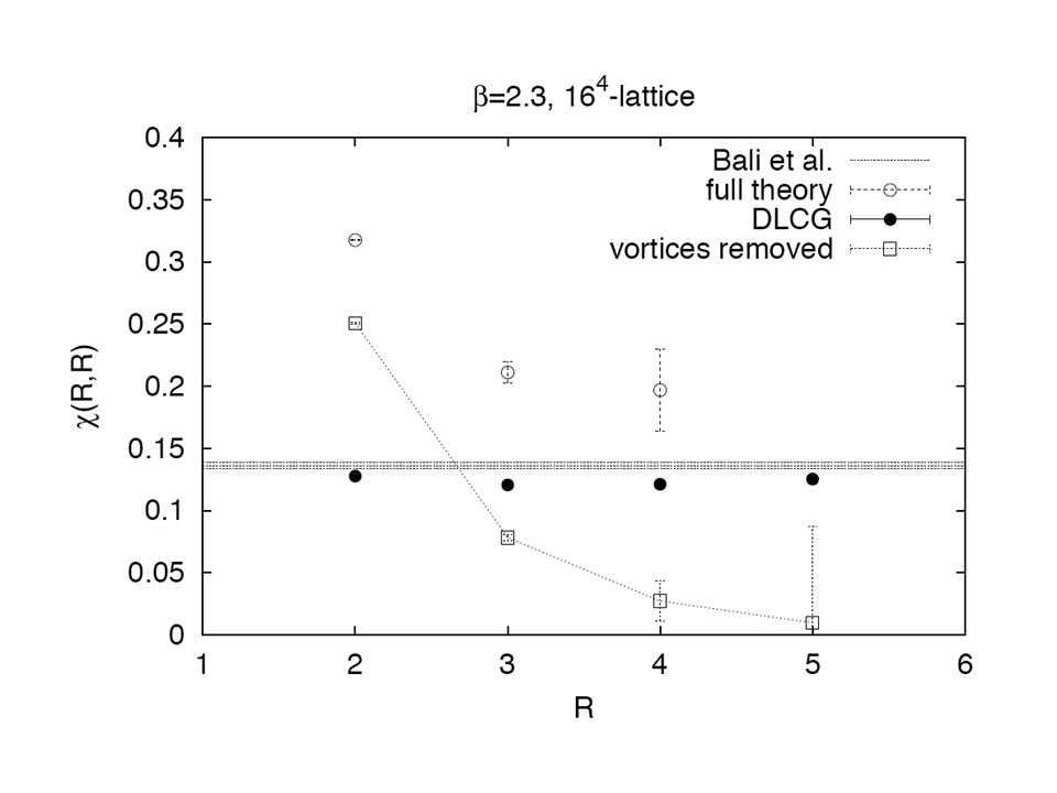

 YM vacuum wave-functional in 2+1 dimensions.>")


Preliminaries: Basic quantities in field theory 2)Preliminaries: COLOUR 3) The QCD Lagrangian.>")
 to a possible change.>")


