Download presentation
Presentation is loading. Please wait.

1
Interest Points and Corners Computer Vision CS 143, Brown James Hays Slides from Rick Szeliski, Svetlana Lazebnik, Derek Hoiem and Grauman&Leibe 2008 AAAI Tutorial Read Szeliski 4.1

2
Correspondence across views Correspondence: matching points, patches, edges, or regions across images ≈

3
Example: estimating “fundamental matrix” that corresponds two views Slide from Silvio Savarese

4
Example: structure from motion

5
Applications Feature points are used for: – Image alignment – 3D reconstruction – Motion tracking – Robot navigation – Indexing and database retrieval – Object recognition

6
This class: interest points Note: “interest points” = “keypoints”, also sometimes called “features” Many applications – tracking: which points are good to track? – recognition: find patches likely to tell us something about object category – 3D reconstruction: find correspondences across different views

7
This class: interest points Suppose you have to click on some point, go away and come back after I deform the image, and click on the same points again. – Which points would you choose? original deformed

8
Overview of Keypoint Matching K. Grauman, B. Leibe B1B1 B2B2 B3B3 A1A1 A2A2 A3A3 1. Find a set of distinctive key- points 3. Extract and normalize the region content 2. Define a region around each keypoint 4. Compute a local descriptor from the normalized region 5. Match local descriptors

9
Goals for Keypoints Detect points that are repeatable and distinctive

10
Key trade-offs More Repeatable More Points B1B1 B2B2 B3B3 A1A1 A2A2 A3A3 Detection of interest points More Distinctive More Flexible Description of patches Robust to occlusion Works with less texture Minimize wrong matches Robust to expected variations Maximize correct matches Robust detection Precise localization

11
Invariant Local Features Image content is transformed into local feature coordinates that are invariant to translation, rotation, scale, and other imaging parameters Features Descriptors

12
Choosing distinctive interest points If you wanted to meet a friend would you say a)“Let’s meet on campus.” b)“Let’s meet on Green street.” c)“Let’s meet at Green and Wright.” – Corner detection Or if you were in a secluded area: a)“Let’s meet in the Plains of Akbar.” b)“Let’s meet on the side of Mt. Doom.” c)“Let’s meet on top of Mt. Doom.” – Blob (valley/peak) detection
 Let’s meet on top of Mt. Doom. – Blob (valley/peak) detection.")
13
Choosing interest points Where would you tell your friend to meet you?

14
Choosing interest points Where would you tell your friend to meet you?

15
Feature extraction: Corners 9300 Harris Corners Pkwy, Charlotte, NC Slides from Rick Szeliski, Svetlana Lazebnik, and Kristin Grauman

16
Why extract features? Motivation: panorama stitching We have two images – how do we combine them?

17
Local features: main components 1)Detection: Identify the interest points 2)Description : Extract vector feature descriptor surrounding each interest point. 3)Matching: Determine correspondence between descriptors in two views Kristen Grauman
Matching: Determine correspondence between descriptors in two views Kristen Grauman.")
18
Characteristics of good features Repeatability The same feature can be found in several images despite geometric and photometric transformations Saliency Each feature is distinctive Compactness and efficiency Many fewer features than image pixels Locality A feature occupies a relatively small area of the image; robust to clutter and occlusion

19
Goal: interest operator repeatability We want to detect (at least some of) the same points in both images. Yet we have to be able to run the detection procedure independently per image. No chance to find true matches! Kristen Grauman

20
Goal: descriptor distinctiveness We want to be able to reliably determine which point goes with which. Must provide some invariance to geometric and photometric differences between the two views. ? Kristen Grauman

21
Local features: main components 1)Detection: Identify the interest points 2)Description :Extract vector feature descriptor surrounding each interest point. 3)Matching: Determine correspondence between descriptors in two views
Matching: Determine correspondence between descriptors in two views.")
22
Many Existing Detectors Available K. Grauman, B. Leibe Hessian & Harris [Beaudet ‘78], [Harris ‘88] Laplacian, DoG [Lindeberg ‘98], [Lowe 1999] Harris-/Hessian-Laplace [Mikolajczyk & Schmid ‘01] Harris-/Hessian-Affine [Mikolajczyk & Schmid ‘04] EBR and IBR [Tuytelaars & Van Gool ‘04] MSER [Matas ‘02] Salient Regions [Kadir & Brady ‘01] Others…

23
What points would you choose? Kristen Grauman

24
Corner Detection: Basic Idea We should easily recognize the point by looking through a small window Shifting a window in any direction should give a large change in intensity “edge”: no change along the edge direction “corner”: significant change in all directions “flat” region: no change in all directions Source: A. Efros

25
Finding Corners Key property: in the region around a corner, image gradient has two or more dominant directions Corners are repeatable and distinctive C.Harris and M.Stephens. "A Combined Corner and Edge Detector.“ Proceedings of the 4th Alvey Vision Conference: pages 147--151. "A Combined Corner and Edge Detector.“

26
Corner Detection: Mathematics Change in appearance of window w(x,y) for the shift [u,v]: I(x, y) E(u, v) E(3,2) w(x, y)
![Corner Detection: Mathematics Change in appearance of window w(x,y) for the shift [u,v]: I(x, y) E(u, v) E(3,2) w(x, y)](http://images.slideplayer.com/16/5088680/slides/slide_26.jpg "Corner Detection: Mathematics Change in appearance of window w(x,y) for the shift [u,v]: I(x, y) E(u, v) E(3,2) w(x, y)")
27
Corner Detection: Mathematics I(x, y) E(u, v) E(0,0) w(x, y) Change in appearance of window w(x,y) for the shift [u,v]:
![Corner Detection: Mathematics I(x, y) E(u, v) E(0,0) w(x, y) Change in appearance of window w(x,y) for the shift [u,v]:](http://images.slideplayer.com/16/5088680/slides/slide_27.jpg "Corner Detection: Mathematics I(x, y) E(u, v) E(0,0) w(x, y) Change in appearance of window w(x,y) for the shift [u,v]:")
28
Corner Detection: Mathematics Intensity Shifted intensity Window function or Window function w(x,y) = Gaussian1 in window, 0 outside Source: R. Szeliski Change in appearance of window w(x,y) for the shift [u,v]:
 for the shift [u,v]:.")
29
Corner Detection: Mathematics We want to find out how this function behaves for small shifts Change in appearance of window w(x,y) for the shift [u,v]: E(u, v)
![Corner Detection: Mathematics We want to find out how this function behaves for small shifts Change in appearance of window w(x,y) for the shift [u,v]: E(u, v)](http://images.slideplayer.com/16/5088680/slides/slide_29.jpg "Corner Detection: Mathematics We want to find out how this function behaves for small shifts Change in appearance of window w(x,y) for the shift [u,v]: E(u, v)")
30
Corner Detection: Mathematics Local quadratic approximation of E(u,v) in the neighborhood of (0,0) is given by the second-order Taylor expansion: We want to find out how this function behaves for small shifts Change in appearance of window w(x,y) for the shift [u,v]:
![Corner Detection: Mathematics Local quadratic approximation of E(u,v) in the neighborhood of (0,0) is given by the second-order Taylor expansion: We want to find out how this function behaves for small shifts Change in appearance of window w(x,y) for the shift [u,v]:](http://images.slideplayer.com/16/5088680/slides/slide_30.jpg "Corner Detection: Mathematics Local quadratic approximation of E(u,v) in the neighborhood of (0,0) is given by the second-order Taylor expansion: We want to find out how this function behaves for small shifts Change in appearance of window w(x,y) for the shift [u,v]:")
31
Corner Detection: Mathematics Second-order Taylor expansion of E(u,v) about (0,0):
 about (0,0):")
32
Corner Detection: Mathematics Second-order Taylor expansion of E(u,v) about (0,0):
 about (0,0):")
33
Corner Detection: Mathematics Second-order Taylor expansion of E(u,v) about (0,0):
 about (0,0):")
34
Corner Detection: Mathematics The quadratic approximation simplifies to where M is a second moment matrix computed from image derivatives: M

35
Corners as distinctive interest points 2 x 2 matrix of image derivatives (averaged in neighborhood of a point). Notation:

36
The surface E(u,v) is locally approximated by a quadratic form. Let’s try to understand its shape. Interpreting the second moment matrix

37
First, consider the axis-aligned case (gradients are either horizontal or vertical) If either λ is close to 0, then this is not a corner, so look for locations where both are large. Interpreting the second moment matrix

38
Consider a horizontal “slice” of E(u, v): Interpreting the second moment matrix This is the equation of an ellipse.
: Interpreting the second moment matrix This is the equation of an ellipse.")
39
Consider a horizontal “slice” of E(u, v): Interpreting the second moment matrix This is the equation of an ellipse. The axis lengths of the ellipse are determined by the eigenvalues and the orientation is determined by R direction of the slowest change direction of the fastest change ( max ) -1/2 ( min ) -1/2 Diagonalization of M:
 -1/2 ( min ) -1/2 Diagonalization of M:.")
40
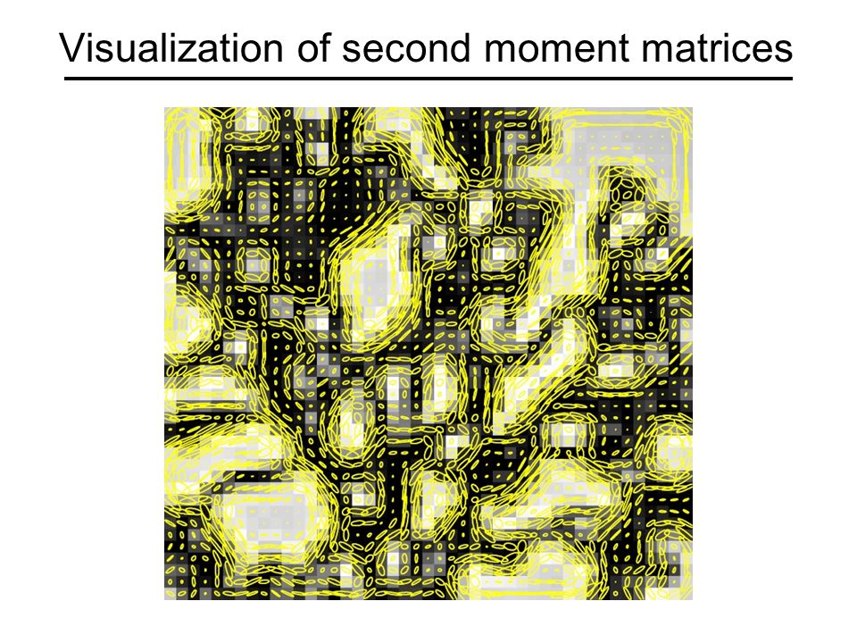
Visualization of second moment matrices

42
Interpreting the eigenvalues 1 2 “Corner” 1 and 2 are large, 1 ~ 2 ; E increases in all directions 1 and 2 are small; E is almost constant in all directions “Edge” 1 >> 2 “Edge” 2 >> 1 “Flat” region Classification of image points using eigenvalues of M:

43
Corner response function “Corner” R > 0 “Edge” R < 0 “Flat” region |R| small α : constant (0.04 to 0.06)
")
44
Harris corner detector 1)Compute M matrix for each image window to get their cornerness scores. 2)Find points whose surrounding window gave large corner response (f> threshold) 3)Take the points of local maxima, i.e., perform non-maximum suppression C.Harris and M.Stephens. “A Combined Corner and Edge Detector.” Proceedings of the 4th Alvey Vision Conference: pages 147—151, 1988. “A Combined Corner and Edge Detector.”
Find points whose surrounding window gave large corner response (f> threshold) 3)Take the points of local maxima, i.e., perform non-maximum suppression C.Harris and M.Stephens. A Combined Corner and Edge Detector. Proceedings of the 4th Alvey Vision Conference: pages 147—151, A Combined Corner and Edge Detector. .")
45
Harris Detector [ Harris88 ] Second moment matrix 45 1. Image derivatives 2. Square of derivatives 3. Gaussian filter g( I ) IxIx IyIy Ix2Ix2 Iy2Iy2 IxIyIxIy g(I x 2 )g(I y 2 ) g(I x I y ) 4. Cornerness function – both eigenvalues are strong har 5. Non-maxima suppression (optionally, blur first)
![Harris Detector [ Harris88 ] Second moment matrix 45 1.](http://images.slideplayer.com/16/5088680/slides/slide_45.jpg "Image derivatives 2. Square of derivatives 3. Gaussian filter g( I ) IxIx IyIy Ix2Ix2 Iy2Iy2 IxIyIxIy g(I x 2 )g(I y 2 ) g(I x I y ) 4. Cornerness function – both eigenvalues are strong har 5. Non-maxima suppression (optionally, blur first).")
46
Harris Detector: Steps

47
Compute corner response R

48
Harris Detector: Steps Find points with large corner response: R>threshold

49
Harris Detector: Steps Take only the points of local maxima of R

50
Harris Detector: Steps

51
Invariance and covariance We want corner locations to be invariant to photometric transformations and covariant to geometric transformations Invariance: image is transformed and corner locations do not change Covariance: if we have two transformed versions of the same image, features should be detected in corresponding locations

52
Affine intensity change Only derivatives are used => invariance to intensity shift I I + b Intensity scaling: I a I R x (image coordinate) threshold R x (image coordinate) Partially invariant to affine intensity change I a I + b
 threshold R x (image coordinate) Partially invariant to affine intensity change I a I + b")
53
Image translation Derivatives and window function are shift-invariant Corner location is covariant w.r.t. translation

54
Image rotation Second moment ellipse rotates but its shape (i.e. eigenvalues) remains the same Corner location is covariant w.r.t. rotation
 remains the same Corner location is covariant w.r.t. rotation.")
55
Scaling All points will be classified as edges Corner Corner location is not covariant to scaling!

56
Next Lecture How do we represent the patches around the interest points? How do we make sure that representation is invariant?

Similar presentations


>")


 15-463: Computational Photography Alexei Efros, CMU, Fall 2005 with a lot of slides stolen from Steve Seitz and.>")

 Generally useful patterns (edges) Also (new) “Interesting” distinctive patterns ( No specific pattern:>")

 15-463: Computational Photography Alexei Efros, CMU, Fall 2006 with a lot of slides stolen from Steve Seitz and.>")


>")