1. CS 460 Spring 2011 Lecture 3 Heuristic Search / Local Search

2. Review Problem-solving agent design and implementation – PEAS Vacuum cleaner world Problem solving as search – State space (abstraction), problem statement, goal, solution Search: tree search, graph search, Search strategies – Uninformed vs informed – Graph vs. Tree: keep track of nodes already explored Uninformed – BFS, Uniform-cost, DFS + variant Evaluation of strategies – Completeness, time complexity, space complexity, optimality

3. Review: Tree search A search strategy is defined by picking the order of node expansion

5. Graph Search

6. Informed search algorithms Chapter 3 & 4

7. Material 3.5.1, 3.5.2, 3.6, 4.1

8. Outline Best-first search Greedy best-first search A * search Heuristics Local search algorithms Hill-climbing search Simulated annealing search Local beam search Genetic algorithms

9. Informed Search Use additional information about problem to guide the search E.g., in Romanian travel problem, estimated distance from a node to destination as the crow flies “heuristic”

10. Best-first search Idea: use an evaluation function f(n) for each node – estimate of "desirability"  Expand most desirable unexpanded node Implementation: – Order the nodes in fringe (frontier in ed 3) in decreasing order of desirability – Compare with uniform cost strategy Special cases: – greedy best-first search – A * search

11. Romania with step costs in km

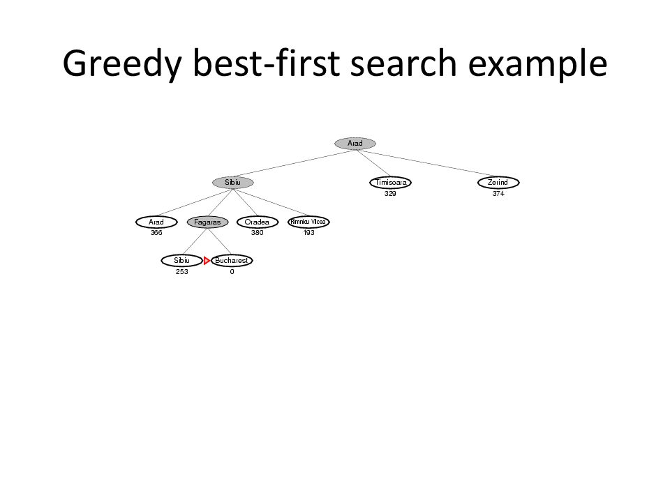
12. Greedy best-first search Evaluation function f(n) = h(n) (heuristic) = estimate of cost from n to goal e.g., h SLD (n) = straight-line distance from n to Bucharest Greedy best-first search expands the node that appears to be closest to goal

13. Greedy best-first search example

17. Greedy BeFS vs Uniform Cost

18. Properties of greedy best-first search Complete? No – can get stuck in loops, e.g., Iasi  Neamt  Iasi  Neamt  (from Iasi to Fagaras, using tree search) Time? O(b m ), but a good heuristic can give dramatic improvement Space? O(b m ) -- keeps all nodes in memory Optimal? No – (shorter to go to Bucharest through Rimnicu Vilcea  Pitesti)

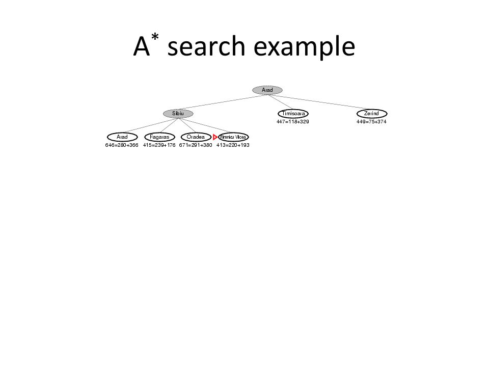
19. A * search Idea: avoid expanding paths that are already expensive Evaluation function f(n) = g(n) + h(n) g(n) = cost so far to reach n h(n) = estimated cost from n to goal f(n) = estimated total cost of path through n to goal Compare with uniform cost search – Uses ony g(n)

20. A * search example

26. Admissible heuristics A heuristic h(n) is admissible if for every node n, h(n) ≤ h * (n), where h * (n) is the true cost to reach the goal state from n. An admissible heuristic never overestimates the cost to reach the goal, i.e., it is optimistic (SLD uses triangle inequality) By trying to achieve a underestimate of the cost, you get close to achieving optimal cost Example: h SLD (n) (never overestimates the actual road distance) Theorem: If h(n) is admissible, A * using TREE-SEARCH is optimal

27. Optimality of A * (proof) Suppose some suboptimal goal G 2 has been generated and is in the fringe. Let n be an unexpanded node in the fringe such that n is on a shortest path to an optimal goal G. f(G 2 ) = g(G 2 )since h(G 2 ) = 0 g(G 2 ) > g(G) since G 2 is suboptimal f(G) = g(G)since h(G) = 0 f(G 2 ) > f(G)from above

28. Optimality of A * (proof) Suppose some suboptimal goal G 2 has been generated and is in the fringe. Let n be an unexpanded node in the fringe such that n is on a shortest path to an optimal goal G. f(G 2 )> f(G) from above h(n)≤ h^*(n)since h is admissible g(n) + h(n)≤ g(n) + h * (n) f(n) ≤ f(G) Hence f(G 2 ) > f(n), and A * will never select G 2 for expansion

29. Consistent heuristics A heuristic is consistent if for every node n, every successor n' of n generated by any action a, h(n) ≤ c(n,a,n') + h(n') If h is consistent, we have f(n') = g(n') + h(n') = g(n) + c(n,a,n') + h(n') ≥ g(n) + h(n) = f(n) i.e., f(n) is non-decreasing along any path. (start with lowest optimistic estimate, then ‘sacrifice’ some optimality at every step taken) Theorem: If h(n) is consistent, A* using GRAPH-SEARCH is optimal

30. Optimality of A * A * expands nodes in order of increasing f value Gradually adds "f-contours" of nodes Contour i has all nodes with f=f i, where f i < f i+1

31. Properties of A$^*$ Complete? Yes (unless there are infinitely many nodes with f ≤ f(G) ) Time? Exponential Space? Keeps all nodes in memory Optimal? Yes Heuristics are needed to make time and space manageable

32. Admissible heuristics E.g., for the 8-puzzle: h 1 (n) = number of misplaced tiles h 2 (n) = total Manhattan distance (i.e., no. of squares from desired location of each tile) h 1 (S) = ? h 2 (S) = ?

33. Admissible heuristics E.g., for the 8-puzzle: h 1 (n) = number of misplaced tiles h 2 (n) = total Manhattan distance (i.e., no. of squares from desired location of each tile) h 1 (S) = ? 8 h 2 (S) = ? 3+1+2+2+2+3+3+2 = 18

34. Dominance If h 2 (n) ≥ h 1 (n) for all n (both admissible) then h 2 dominates h 1 h 2 is better for search Typical search costs (average number of nodes expanded): d=12IDS = 3,644,035 nodes A * (h 1 ) = 227 nodes A * (h 2 ) = 73 nodes d=24 IDS = too many nodes A * (h 1 ) = 39,135 nodes A * (h 2 ) = 1,641 nodes

35. Relaxed problems A problem with fewer restrictions on the actions is called a relaxed problem The cost of an optimal solution to a relaxed problem is an admissible heuristic for the original problem If the rules of the 8-puzzle are relaxed so that a tile can move anywhere, then h 1 (n) gives the shortest solution If the rules are relaxed so that a tile can move to any adjacent square, then h 2 (n) gives the shortest solution

36. Local search algorithms In many optimization problems, the path to the goal is irrelevant; the goal state itself is the solution State space = set of "complete" configurations Find configuration satisfying constraints, e.g., n- queens In such cases, we can use local search algorithms keep a single "current" state, try to improve it – Thus also address memory limitations of heuristic searches

37. Example: n-queens Put n queens on an n × n board with no two queens on the same row, column, or diagonal

38. Hill-climbing search "Like climbing Everest in thick fog with amnesia"

39. Hill-climbing search Problem: depending on initial state, can get stuck in local maxima

40. Hill-climbing search: 8-queens problem h = number of pairs of queens that are attacking each other, either directly or indirectly h = 17 for the above state

41. 8 queens succ: move a single queen to another square in same column Each state has 8 x 7 = 56 successor states Number in each square represents total number of attack pairs for the state resulting when queen in that column is moved to that square Choose randomly among ‘best’ successors if there is more than one Greedy local search – Doesn’t always get to the global optimum, only local – In the example, we get to h=1 in 5 moves but can’t do better – Local maxima, ridges, plateaux – Use sideways moves, have to cutoff to avoid infinite loops

42. Hill-climbing search: 8-queens problem A local minimum with h = 1

43. Hill climbing Steepest ascent HC Stochastic HC – First choice HC Random restart HC Hill climbing algorithms are usually incomplete – Guaranteed to be incomplete if no downhill moves But, with effective variants, HC can converge quite fast to a solution 8^8 states for 8 queens – Can solve in about 22 steps on average Can find solution in under a minute for 3M queens

44. Simulated annealing search Idea: escape local maxima by allowing some "bad" moves but gradually decrease their frequency

45. Properties of simulated annealing search One can prove: If T decreases slowly enough, then simulated annealing search will find a global optimum with probability approaching 1 Widely used in VLSI layout, airline scheduling, etc

46. Local beam search Keep track of k states rather than just one Start with k randomly generated states At each iteration, all the successors of all k states are generated If any one is a goal state, stop; else select the k best successors from the complete list and repeat.

47. Genetic algorithms A successor state is generated by combining two parent states Start with k randomly generated states (population) A state is represented as a string over a finite alphabet (often a string of 0s and 1s) Evaluation function (fitness function). Higher values for better states. Produce the next generation of states by selection, crossover, and mutation

48. Genetic algorithms Fitness function: number of non-attacking pairs of queens (min = 0, max = 8 × 7/2 = 28) 24/(24+23+20+11) = 31% 23/(24+23+20+11) = 29% etc

49. Genetic algorithms