1. Chapter 11: Scheduling Real- Time Systems
Real-Time Systems and Programming Languages © Alan Burns and Andy Wellings

2. Aims
To understand the role that scheduling and schedulability analysis plays in predicting that real-time applications meet their deadlines
To understand the cyclic executive approach and its limitations
To introduce process-based scheduling and distinguish between the various approaches available

3. Aims To introduce Rate Monotonic priority assignment
To introduce utilization-based schedulability test
To show why utilization-based necessary are sufficient but not necessary
To provide and introduction to response time analysis for Fixed Priority scheduling
Proof of Deadline Monotonic Priority Ordering optimality

4. Aims
To understand how response time analysis can be extended to cope with blocking of resources
To explain priority inversion, priority inheritance and ceiling protocols
To show that response-time analysis is flexible enough to cope with many application demands by simple extensions
To cover Earliest Deadline First (EDF) scheduling

5. Aims To briefly consider dynamic scheduling
To provide an overview of the issues related to Worst-Case Execution Time (WCET) analysis
Consideration of multiprocessor scheduling
Consideration of power-aware scheduling
System overhead estimation

6. Scheduling In general, a scheduling scheme provides two features:
An algorithm for ordering the use of system resources (in particular the CPUs)
A means of predicting the worst-case behaviour of the system when the scheduling algorithm is applied
The prediction can then be used to confirm the temporal requirements of the application

7. Cyclic Executives
One common way of implementing hard real-time systems is to use a cyclic executive
Here the design is concurrent but the code is produced as a collection of procedures
Procedures are mapped onto a set of minor cycles that constitute the complete schedule (or major cycle)
Minor cycle dictates the minimum cycle time
Major cycle dictates the maximum cycle time
Has the advantage of being fully deterministic

8. Consider Task Set Task Period,T Computation Time,C a 25 10 b 25 8

9. Time-line for Task Set Interrupt Interrupt Interrupt Interrupt a b c ad e a b c

10. Properties
No actual tasks exist at run-time; each minor cycle is just a sequence of procedure calls
The procedures share a common address space and can thus pass data between themselves. This data does not need to be protected (via a semaphore, for example) because concurrent access is not possible

11. Problems with Cyclic Exec.
All “task” periods must be a multiple of the minor cycle time
The difficulty of incorporating tasks with long periods; the major cycle time is the maximum period that can be accommodated without secondary schedules
Sporadic activities are difficult (impossible!) to incorporate
The cyclic executive is difficult to construct and difficult to maintain — it is a NP-hard problem

12. Problems with Cyclic Exec.
Any “task” with a sizable computation time will need to be split into a fixed number of fixed sized procedures (this may cut across the structure of the code from a software engineering perspective, and hence may be error-prone)
More flexible scheduling methods are difficult to support
Determinism is not required, but predictability is

13. Task-Based Scheduling
Tasks exist at run-time
Supported by real-time OS or run-time
Each task is:
Runnable (and possible running), or
Suspended waiting for a timing event
Suspended waiting for a non-timing event

14. Task-Based Scheduling
Scheduling approaches
Fixed-Priority Scheduling (FPS)
Earliest Deadline First (EDF)
Value-Based Scheduling (VBS)

15. Fixed-Priority Scheduling (FPS)
This is the most widely used approach and is the main focus of this course
Each task has a fixed, static, priority which is computer pre-run-time
The runnable tasks are executed in the order determined by their priority
In real-time systems, the “priority” of a task is derived from its temporal requirements, not its importance to the correct functioning of the system or its integrity

16. Earliest Deadline First (EDF)
The runnable tasks are executed in the order determined by the absolute deadlines of the tasks
The next task to run being the one with the shortest (nearest) deadline
Although it is usual to know the relative deadlines of each task (e.g. 25ms after release), the absolute deadlines are computed at run time and hence the scheme is described as dynamic

17. Value-Based Scheduling (VBS)
If a system can become overloaded then the use of simple static priorities or deadlines is not sufficient; a more adaptive scheme is needed
This often takes the form of assigning a value to each task and employing an on-line value-based scheduling algorithm to decide which task to run next

18. Preemption
With priority-based scheduling, a high-priority task may be released during the execution of a lower priority one
In a preemptive scheme, there will be an immediate switch to the higher-priority task
With non-preemption, the lower-priority task will be allowed to complete before the other executes
Preemptive schemes enable higher-priority tasks to be more reactive, and hence they are preferred
Cooperative dispatching (deferred preemption) is a half-way house
Schemes such as EDF and VBS can also take on a pre-emptive or non pre-emptive form

19. Scheduling Characteristics
Sufficient – pass the test will meet deadlines
Necessary – fail the test will miss deadlines
Exact – necessary and sufficient
Sustainable – system stays schedulable if conditions ‘improve’

20. Simple Task Model
The application is assumed to consist of a fixed set of tasks
All tasks are periodic, with known periods
The tasks are completely independent of each other
All system's overheads, context-switching times and so on are ignored (i.e, assumed to have zero cost)
All tasks have a deadline equal to their period (that is, each task must complete before it is next released)
All tasks have a fixed worst-case execution time

21. Standard Notation B C D I J N P R T U a-z
Worst-case blocking time for the task (if applicable)
Worst-case computation time (WCET) of the task
Deadline of the task
The interference time of the task
Release jitter of the task
Number of tasks in the system
Priority assigned to the task (if applicable)
Worst-case response time of the task
Minimum time between task releases, jobs, (task period)
The utilization of each task (equal to C/T)
The name of a task

22. Rate Monotonic Priority Assignment
Each task is assigned a (unique) priority based on its period; the shorter the period, the higher the priority
i.e, for two tasks i and j,
This assignment is optimal in the sense that if any task set can be scheduled (using pre-emptive priority-based scheduling) with a fixed-priority assignment scheme, then the given task set can also be scheduled with a rate monotonic assignment scheme
Note, priority 1 is the lowest (least) priority

23. Example Priority Assignment
Process Period, T Priority, P a b c d e

24. Utilization-Based Analysis
For D=T task sets only
A simple sufficient but not necessary schedulability test exists

25. Utilization Bounds N Utilization bound 1 100.0% 2 82.8% 3 78.0%% % % % % %
Approaches 69.3% asymptotically

26. Task Set A Task Period ComputationTime Priority Utilization T C P Ub c
The combined utilization is 0.82 (or 82%)
This is above the threshold for three tasks (0.78) and, hence, this task set fails the utilization test

27. Time-line for task Set A
Task Release Time
Task Completion Time
Deadline Met b
Task Completion Time
Deadline Missed
Preempted c
Executing 10 20 30 40 50 60
Time

28. Gantt Chart for Task Set Ab a c b 10 20 30 40 50
Time

29. Task Set B Task Period ComputationTime Priority Utilization T C P U
The combined utilization is 0.775
This is below the threshold for three tasks (0.78) and, hence, this task set will meet all its deadlines

30. Task Set C Task Period ComputationTime Priority Utilization T C P Ub c
The combined utilization is 1.0
This is above the threshold for three tasks (0.78) but the task set will meet all its deadlines

31. Time-line for Task Set Cb c 10 20 30 40 50 60 70 80
Time

32. Improved Tests - I Use families of task (N stands for families), so
In Task Set B, let period of Task c change to 14
Now utilisation is approximately 0.81
Above L&L threshold for 3 tasks
But period of a is same as period of b, so N=2
L&L bound for N=2 is 0.828

33. Improved Tests - II
Alternative formulae

34. Criticism of Tests Not exact Not general BUT it is O(N)
The test is sufficient but not necessary

35. Response-Time Analysis
Here task i's worst-case response time, R, is calculated first and then checked (trivially) with its deadline
Where I is the interference from higher priority tasks

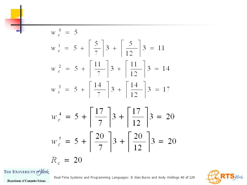
36. Calculating R
During R, each higher priority task j will execute a number of times:
The ceiling function gives the smallest integer greater than the fractional number on which it acts. So the ceiling of 1/3 is 1, of 6/5 is 2, and of 6/3 is 2.
Total interference is given by:

37. Response Time Equation
Where hp(i) is the set of tasks with priority higher than task i
Solve by forming a recurrence relationship:
The set of values is monotonically non decreasing.
When the solution to the equation has been found;
must not be greater that (e.g. 0 or )

38. Response Time Algorithm
for i in 1..N loop -- for each process in turn
n := 0
loop
calculate new
if then
exit value found
end if
exit value not found
n := n + 1
end loop

39. Task Set D Task Period ComputationTime Priority T C P a 7 3 3 b 12 3 2

41. Revisit: Task Set C
Process Period ComputationTime Priority Response time
T C P R a b c
The combined utilization is 1.0
This was above the utilization threshold for three tasks (0.78), therefore it failed the test
The response time analysis shows that the task set will meet all its deadlines

42. Response Time Analysis
Is sufficient and necessary (exact)
If the task set passes the test they will meet all their deadlines; if they fail the test then, at run-time, a task will miss its deadline (unless the computation time estimations themselves turn out to be pessimistic)

43. Sporadic Tasks Sporadics tasks have a minimum inter-arrival time
They also require D<T
The response time algorithm for fixed priority scheduling works perfectly for values of D less than T as long as the stopping criteria becomes
It also works perfectly well with any priority ordering — hp(i) always gives the set of higher-priority tasks

44. Hard and Soft Tasks
In many situations the worst-case figures for sporadic tasks are considerably higher than the averages
Interrupts often arrive in bursts and an abnormal sensor reading may lead to significant additional computation
Measuring schedulability with worst-case figures may lead to very low processor utilizations being observed in the actual running system

45. General Guidelines
Rule 1 — all tasks should be schedulable using average execution times and average arrival rates
Rule 2 — all hard real-time tasks should be schedulable using worst-case execution times and worst-case arrival rates of all tasks (including soft)
A consequent of Rule 1 is that there may be situations in which it is not possible to meet all current deadlines
This condition is known as a transient overload
Rule 2 ensures that no hard real-time task will miss its deadline
If Rule 2 gives rise to unacceptably low utilizations for “normal execution” then action must be taken to reduce the worst-case execution times (or arrival rates)

46. Aperiodic Tasks These do not have minimum inter-arrival times
Can run aperiodic tasks at a priority below the priorities assigned to hard processes, therefore, they cannot steal, in a pre-emptive system, resources from the hard processes
This does not provide adequate support to soft tasks which will often miss their deadlines
To improve the situation for soft tasks, a server can be employed

47. Execution-time Servers
A server:
Has a capacity/budget of C that is available to its client tasks (typically aperiodic tasks)
When a client runs it uses up the budget
The server has a replenishment policy
If there is currently no budget then clients do not run
Hence it protects other tasks from excessive aperiodic activity

48. Periodic Server (PS) Budget C
Replenishment Period T, starting at say 0
Client ready to run at time 0 (or T, 2T etc) runs while budget available, is then suspended
Budget ‘idles away’ if no clients

49. Deferrable Server (DS)
Budget C
Period T – replenished every T time units (back to C)
For example 10ms every 50ms
Anytime budget available clients can execute
Client suspended when budget exhausted
DS and SS are referred to as bandwidth preserving
Retain capacity as long as possible
PS is not bandwidth preserving

50. Sporadic Server (SS)
Initially defined to enforce minimum separation for sporadic tasks
Parameters C and T
Request at time t (for a < C) is accepted
a is returned to server at time t+T
Request at time t (for 2C>A>C):
C available immediately
Replenished at time t+T
Remainder (2C-A) available at this time

51. Task Sets with D < T
For D = T, Rate Monotonic priority ordering is optimal
For D < T, Deadline Monotonic priority ordering is optimal

52. D < T Example Task Set
Task Period Deadline ComputationTime Priority Response time
T D C P R a b c d

53. Proof that DMPO is Optimal
Deadline monotonic priority ordering (DMPO) is optimal if any task set, Q, that is schedulable by priority scheme, W, is also schedulable by DMPO
The proof of optimality of DMPO involves transforming the priorities of Q (as assigned by W) until the ordering is DMPO
Each step of the transformation will preserve schedulability

54. DMPO Proof Continued
Let i and j be two tasks (with adjacent priorities) in Q such that under W:
Define scheme W’ to be identical to W except that tasks i and j are swapped
Consider the schedulability of Q under W’
All tasks with priorities greater than will be unaffected by this change to lower-priority tasks
All tasks with priorities lower than will be unaffected; they will all experience the same interference from i and j
Task j, which was schedulable under W, now has a higher priority, suffers less interference, and hence must be schedulable under W’

55. DMPO Proof Continued
All that is left is the need to show that task i, which has had its priority lowered, is still schedulable
Under W
Hence task i only interferes once during the execution of j
It follows that:
It can be concluded that task i is schedulable after the switch
Priority scheme W’ can now be transformed to W" by choosing two more tasks that are in the wrong order for DMP and switching them

56. Task Interactions and Blocking
If a task is suspended waiting for a lower-priority task to complete some required computation then the priority model is, in some sense, being undermined
It is said to suffer priority inversion
If a task is waiting for a lower-priority task, it is said to be blocked

57. Priority Inversion
To illustrate an extreme example of priority inversion, consider the executions of four periodic tasks: a, b, c and d; and two resources: Q and V
Task Priority Execution Sequence Release Time
a EQQQQE
b EE
c EVVE
d EEQVE

58. Example of Priority Inversiond c b a 2 4 6 8 10 12 14 16 18

59. Symbols Executing Executing Preempted Preempted
Executing with Q locked
Executing with Q locked
Blocked
Blocked
Executing with V locked

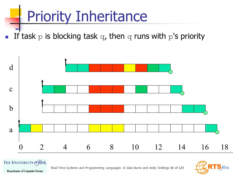
60. Priority Inheritance
If task p is blocking task q, then q runs with p's priority d c b a 2 4 6 8 10 12 14 16 18

61. Mars Path-Finder
A problem due to priority inversion nearly caused the lose of the Mars Path-finder mission
As a shared bus got heavily loaded critical data was not been transferred
Time-out on this data was used as an indication of failure and lead to re-boot
Solution was a patch that turned on priority inheritance, this solved the problem

62. Calculating Blocking
If a task has m critical sections that can lead to it being blocked then the maximum number of times it can be blocked is m
If B is the maximum blocking time and K is the number of critical sections, then task i has an upper bound on its blocking given by:

63. Response Time and Blocking

64. Priority Ceiling Protocols
Two forms
Original ceiling priority protocol
Immediate ceiling priority protocol

65. On a Single Processor
A high-priority task can be blocked at most once during its execution by lower-priority tasks
Deadlocks are prevented
Transitive blocking is prevented
Mutual exclusive access to resources is ensured (by the protocol itself)

66. OCPP
Each task has a static default priority assigned (perhaps by the deadline monotonic scheme)
Each resource has a static ceiling value defined, this is the maximum priority of the tasks that use it
A task has a dynamic priority that is the maximum of its own static priority and any it inherits due to it blocking higher-priority tasks
A task can only lock a resource if its dynamic priority is higher than the ceiling of any currently locked resource (excluding any that it has already locked itself)

67. OCPP Analysis
Even though blocking has a ‘single term’ impact, good design practice is to keen all critical sections small

68. OCPP Inheritance d c b a 2 4 6 8 10 12 14 16 18

69. ICPP
Each task has a static default priority assigned (perhaps by the deadline monotonic scheme)
Each resource has a static ceiling value defined, this is the maximum priority of the tasks that use it
A task has a dynamic priority that is the maximum of its own static priority and the ceiling values of any resources it has locked

70. ICPP - Properties
As a consequence of ICPP, a task will only suffer a block at the very beginning of its execution
Once the task starts actually executing, all the resources it needs must be free; if they were not, then some task would have an equal or higher priority and the task's execution would be postponed

71. ICPP Inheritance d c b a 2 4 6 8 10 12 14 16 18

72. OCPP versus ICPP
Although the worst-case behaviour of the two ceiling schemes is identical (from a scheduling view point), there are some points of difference:
ICCP is easier to implement than the original (OCPP) as blocking relationships need not be monitored
ICPP leads to less context switches as blocking is prior to first execution
ICPP requires more priority movements as this happens with all resource usage
OCPP changes priority only if an actual block has occurred

73. OCPP versus ICPP
Note that ICPP is called Priority Protect Protocol in POSIX and Priority Ceiling Emulation in Real-Time Java

74. An Extendible Task Model
So far:
Deadlines can be less than period (D<T)
Sporadic and aperiodic tasks, as well as periodic tasks, can be supported
Task interactions are possible, with the resulting blocking being factored into the response time equations

75. Extensions Release Jitter Arbitrary Deadlines Cooperative Scheduling
Fault Tolerance
Offsets
Optimal Priority Assignment
Execution-time Servers

76. Release Jitter A key issue for distributed systems
Consider the release of a sporadic task on a different processor by a periodic task, l, with a period of 20
First execution l finishes at R
Second execution of l finishes after C l
Time t
t+15
t+20
Release sporadic process at time 0, 5, 25, 45

77. Release Jitter Sporadic is released at 0, T-J, 2T-J, 3T-J
Examination of the derivation of the schedulability equation implies that task i will suffer
one interference from task s if
two interferences if
three interference if
This can be represented in the response time equations
If response time is to be measured relative to the real release time then the jitter value must be added

78. Arbitrary Deadlines
To cater for situations where D (and hence potentially R) > T
The number of releases is bounded by the lowest value of q for which the following relation is true:
The worst-case response time is then the maximum value found for each q:

79. Arbitrary Deadlines
When formulation is combined with the effect of release jitter, two alterations to the above analysis must be made
First, the interference factor must be increased if any higher priority processes suffers release jitter:
The other change involves the task itself. If it can suffer release jitter then two consecutive windows could overlap if response time plus jitter is greater than period

80. Cooperative Scheduling
True preemptive behaviour is not always acceptable for safety-critical systems
Cooperative or deferred preemption splits tasks into slots
Mutual exclusion is via non-preemption
The use of deferred preemption has two important advantages
It increases the schedulability of the system, and it can lead to lower values of C
With deferred preemption, no interference can occur during the last slot of execution

81. Cooperative Scheduling
Let the execution time of the final block be
When this converges that is, , the response time is given by:

82. BUT - example First task: T=D=6, C=2, F=2 (ie one block)
Second task: T=D=8,C=6, F=3 (2 blocks)
Is this schedulable?
What is utilisation of this task set?

83. Fault Tolerance
Fault tolerance via either forward or backward error recovery always results in extra computation
This could be an exception handler or a recovery block
In a real-time fault tolerant system, deadlines should still be met even when a certain level of faults occur
This level of fault tolerance is know as the fault model
If the extra computation time that results from an error in task i is
where hep(i) is set of tasks with priority equal to or higher than i

84. Fault Tolerance If F is the number of faults allowed
If there is a minimum arrival interval

85. Offsets
So far assumed all tasks share a common release time (critical instant)
Task T D C R a b c
With offsets
Task T D C O R a b c
Arbitrary offsets are not amenable to analysis

86. Non-Optimal Analysis
In most realistic systems, task periods are not arbitrary but are likely to be related to one another
As in the example just illustrated, two tasks have a common period. In these situations it is ease to give one an offset (of T/2) and to analyse the resulting system using a transformation technique that removes the offset — and, hence, critical instant analysis applies
In the example, tasks b and c (having the offset of 10) are replaced by a single notional process with period 10, computation time 4, deadline 10 but no offset

87. Non-Optimal Analysis
Process T D C O R a n

88. Non-Optimal Analysis This notional task has two important properties:
If it is schedulable (when sharing a critical instant with all other tasks) then the two real tasks will meet their deadlines when one is given the half period offset
If all lower priority tasks are schedulable when suffering interference from the notional task (and all other high-priority tasks) then they will remain schedulable when the notional task is replaced by the two real tasks (one with the offset)
These properties follow from the observation that the notional task always uses more (or equal) CPU time than the two real tasks

89. Notional Task Parameters
Can be extended to more than two processes

90. Other Requirements Mode changes Task where C values are variable
Optimal solution not possible for FPS
Where there are gaps in the execution behaviour
Optimal solution not possible for FPS or EDF
Communication protocols
For example CAN
Dual priority

91. Priority Assignment Theorem (Audsley’ algorithm)
If task p is assigned the lowest priority and is feasible then, if a feasible priority ordering exists for the complete task set, an ordering exists with task p assigned the lowest priority

92. Priority Assignment
procedure Assign_Pri (Set : in out Process_Set; N : Natural;
Ok : out Boolean) is
begin
for K in 1..N loop
for Next in K..N loop
Swap(Set, K, Next);
Process_Test(Set, K, Ok);
exit when Ok;
end loop;
exit when not Ok; -- failed to find a schedulable process
end Assign_Pri;

93. Insufficient Priorities
If insufficient priorities then tasks must share priority levels
If task a shares priority with task b, then each must assume the other interferes
Priority assignment algorithm can be used to pack tasks together
Ada requires 31, RT-POSIX 32 and RT-Java 28

94. Execution-time Servers - FPS
Periodic Servers act as periodic tasks
Sporadic Servers act as periodic tasks
Are directly supported by POSIX
Deferrable Servers worst case behaviour is when
Budget available but not used until end of replenishment period
Budget is used, replenished and used again (ie 2C in one go)
Analysed as task with release jitter

95. EDF Scheduling Always run task with earliest absolute deadline
Will consider
Utilisation based tests
Processor demand criteria
QPA
Blocking
Servers

96. Utilization-based Test for EDF
A much simpler test than that for FPS
Superior to FPS (0.69 bound in worst-case); it can support high utilizations. However,
Bound only applicable to simple task model
Although EDF is always as good as FPS, and usually better

97. FPS v EDF FPS is easier to implement as priorities are static
EDF is dynamic and requires a more complex run-time system which will have higher overhead
It is easier to incorporate tasks without deadlines into FPS; giving a task an arbitrary deadline is more artificial
It is easier to incorporate other factors into the notion of priority than it is into the notion of deadline

98. FPS v EDF But EDF gets more out of the processor!
During overload situations
FPS is more predictable; Low priority process miss their deadlines first
EDF is unpredictable; a domino effect can occur in which a large number of processes miss deadlines
But EDF gets more out of the processor!

99. Processor Demand Criteria
Arbitrary EDF system (D less than or greater than T) is schedulable if
Load at time t is less than t, for all t
There is a bound or how big t needs to be
Load expressed as h(t)
Only points in time that refer to actual task deadlines need be checked

100. PDC
If D>T then floor function is constrained to have minimum 0

101. Upper Bound for PDA
U is the utilisation of the task set, note upper bound not
defined for U=1

102. Upper Bound for PDC This is the processor busy period
and is bounded for U no greater
than 1

103. QPA Test Refers to Quick Processor demand Analysis
Start at L, and work backwards towards 0
If at time t, h(t)>t then unschedulable
else let t equal h(t)
If h(t) =t then let t equal t-1 (or smallest absolute deadline <t)
If t < smallest D, then schedulable
Typically QPA requires only 1% of the effort of PDA but is equally necessary and sufficient

104. EDF and Blocking
SRP – Stack Resource Policy – is a generalisation of the priority ceiling protocol
Two notions:
Preemption level for access to shared objects
Urgency for access to processor
With FPS, priority is used for both
With EDF, ‘priority’ is used for preemption level, and earliest absolute deadline is used for urgency

105. EDF and Servers
There are equivalent servers under EDF to those defined for FPS: periodic server, deferrable server and sporadic server
There are also EDF-specific servers
If, for example, an aperiodic task arrives at time 156 and wants 5ms of computation from a server with budget 2ms and period 10ms
Task will need 3 allocations, and hence is given an absolute deadline of 186
EDF scheduling rules are then applied

106. Online Analysis
There are dynamic soft real-time applications in which arrival patterns and computation times are not known a priori
Although some level of offline analysis may still be applicable, this can no longer be complete and hence some form of on-line analysis is required
The main role of an online scheduling scheme is to manage any overload that is likely to occur due to the dynamics of the system's environment
During transient overloads EDF performs very badly. It is possible to get a cascade effect in which each task misses its deadline but uses sufficient resources to result in the next task also missing its deadline

107. Admission Schemes
To counter this detrimental domino effect many on-line schemes have two mechanisms:
an admissions control module that limits the number of tasks that are allowed to compete for the processors, and
an EDF dispatching routine for those tasks that are admitted
An ideal admissions algorithm prevents the processors getting overloaded so that the EDF routine works effectively

108. Values
If some tasks are to be admitted, whilst others rejected, the relative importance of each task must be known
This is usually achieved by assigning value
Values can be classified
Static: the task always has the same value whenever it is released
Dynamic: the task's value can only be computed at the time the task is released (because it is dependent on either environmental factors or the current state of the system)
Adaptive: here the dynamic nature of the system is such that the value of the task will change during its execution

109. Values
To assign static values requires the domain specialists to articulate their understanding of the desirable behaviour of the system

110. Worst-case Execution Time
WCET values are critical for all forms of analysis
C values in all the equations of this chapter
Known as Timing Analysis
Found either by static analysis or measurement
Static analysis is pessimistic and hard to undertake with modern processors with cache(s), pipelines, out-of-order execution, branch prediction etc
Measurement is potentially optimistic – was the worst-case path measured?
Timing analysis usually represents each task as a directed graph of basic blocks (or basic paths)

111. Basic Blocks
Once the worst-case time of each basic block is obtained (via measurement or a model of the processor) then
Direct graph is collapsed with maximum loop parameters and worst-case branches assumed to be taken

112. Example
for i in loop
if Cond then
-- basic block of cost 100
else
-- basic block of cost 10
end if;
end loop;
With no further semantic information must assume total cost is 1000,
But if Cond can only be true 4 times then cost is 460
ILP – Integer Linear Programming – and Constraint Satisfaction
programs are being employed to model basic block dependencies

113. Multiprocessor Issues:
Homogeneous or heterogeneous processors
Globally scheduling or partitioned
Or other alternatives between these two extremes
Optimality?
EDF is not optimal
EDF is not always better than FPS
Global is not always better than partitioned
Partitioning is an allocation problem followed by single processor scheduling

114. Example Task T D C a 10 10 5 2 processors, global b 10 10 5 c 12 12 8
EDF and FPS would run a and b on the 2 processors
No time left for c (7 on each, 14 in total,
but not 8 on one)

115. Example Task T D C d 10 10 9 2 processors, partitioned e 10 10 9f
2 processors, partitioned
Task f can not sit on just one processor, it needs to
migrate and for d and e to cooperate

116. Results For the simple task model introduced earlier
A pfair scheme can theoretically schedule up to a total utilisation of M (for M processors), but overheads are excessive
For FPS with partitioned and first-fit on utilisation
ie 0.414M

117. Results EDF partitioned first-fit
For high maximum utilisation can get lower than 0.25M, but can get close to M for some examples

118. Results
EDF global
Again for high Umax can be as low as 0.2M but also close to M for other examples

119. Results Combinations:
Fixed priority to those tasks with U greater than 0.5
EDF for the rest

120. Power Aware
For battery-power embedded systems it is useful to run the processor with the lowest speed commensurate with meeting all deadlines
Halving the speed may quadruple the life
Sensitivity analysis will, for a schedulable system, enable the maximum scaling factor for all C values to be ascertained – with the system remaining schedulable

121. Overheads
To use in an industrial context, the temporal overheads of implementing the system must be taken in to account
Context switches (one per job)
Interrupts (one per sporadic task release)
Real-time clock overheads
Will consider FPS only here

122. Context switches Rather than
Where the new terms are the cost of switching to
the task and the cost of switching away from the task

123. Interrupt Handling Cost of handling interrupts:
Where is the set of sporadic tasks
And IH is the cost of a single interrupt (which occurs
at maximum priority level)

124. Clocks Overheads There is a cost per clock interrupt
and a cost for moving one task from delay to run queue
and a (reduced) cost of moving groups of tasks
Let be the cost of a single clock interrupt, be the
set of periodic tasks, and be the cost of moving one
task the following equation can be derived

125. Full model

126. Summary
A scheduling scheme defines an algorithm for resource sharing and a means of predicting the worst-case behaviour of an application when that form of resource sharing is used
With a cyclic executive, the application code must be packed into a fixed number of minor cycles such that the cyclic execution of the sequence of minor cycles (the major cycle) will enable all system deadlines to be met
The cyclic executive approach has major drawbacks many of which are solved by priority-based systems

127. Summary
Rate monotonic priority ordering is optimal for the simple task model
Simple utilization-based schedulability tests are not exact for FPS
Response time analysis is flexible and caters for:
Any priority ordering
Periodic and sporadic processes
Is necessary and sufficient for many situations

128. Summary Blocking can result in serious priority inversion
Priority inheritance (in some form) is needed to bound blocking
Priority ceiling protocols bound blocking to a single block, supply mutual exclusion and prevent deadlocks
Response time analysis can easily be extended to cope with blocking caused by ceiling protocols

129. Summary
Examples have been given of how to expand RTA to many different application requirements
RTA is a framework, it must be expanded to deal with particular situations
Analysis of EDF scheduling systems has been covered
Multiprocessor scheduling is still not mature, some current results are outlined
Power aware scheduling was briefly cover
Finally, how to take system overheads into account in response time analysis was addressed