1. Fitting: Concepts and recipes

2. Review: The Hough transform What are the steps of a Hough transform? What line parametrization is best for the Hough transform? How does bin size affect the performance of the Hough transform? What is the complexity of the Hough transform as a function of the number of parameters in the model? How can we use gradient direction to modify the Hough transform? How do we find circles with the Hough transform? What about general shapes?

3. Today: A “grab-bag” of techniques If we know which points belong to the line, how do we find the “optimal” line parameters? Least squares Probabilistic fitting What if there are outliers? Robust fitting, RANSAC What if there are many lines? Incremental fitting, K-lines, EM What if we’re not even sure it’s a line? Model selection Our main case study remains line fitting, but most of the concepts are very generic and widely applicable

4. Least squares line fitting Data: (x 1, y 1 ), …, (x n, y n ) Line equation: y i = m x i + b Find ( m, b ) to minimize (x i, y i ) y=mx+b

5. Least squares line fitting Data: (x 1, y 1 ), …, (x n, y n ) Line equation: y i = m x i + b Find ( m, b ) to minimize Normal equations: least squares solution to XB=Y (x i, y i ) y=mx+b

6. Problem with “vertical” least squares Not rotation-invariant Fails completely for vertical lines

7. Total least squares Distance between point (x n, y n ) and line ax+by=d (a 2 +b 2 =1): |ax + by – d| Find (a, b, d) to minimize the sum of squared perpendicular distances (x i, y i ) ax+by=d Unit normal: N=(a, b)

8. Total least squares Distance between point (x n, y n ) and line ax+by=d (a 2 +b 2 =1): |ax + by – d| Find (a, b, d) to minimize the sum of squared perpendicular distances (x i, y i ) ax+by=d Unit normal: N=(a, b) Solution to ( U T U)N = 0, subject to ||N|| 2 = 1 : eigenvector of U T U associated with the smallest eigenvalue (least squares solution to homogeneous linear system UN = 0 )

9. Total least squares second moment matrix

10. Total least squares N = (a, b) second moment matrix

11. Least squares as likelihood maximization Generative model: line points are corrupted by Gaussian noise in the direction perpendicular to the line (x, y) ax+by=d (u, v) ε point on the line noise: zero-mean Gaussian with std. dev. σ normal direction

12. Least squares as likelihood maximization Generative model: line points are corrupted by Gaussian noise in the direction perpendicular to the line (x, y) (u, v) ε Likelihood of points given line parameters (a, b, d): Log-likelihood: ax+by=d

13. Probabilistic fitting: General concepts Likelihood:

14. Probabilistic fitting: General concepts Likelihood: Log-likelihood:

15. Probabilistic fitting: General concepts Likelihood: Log-likelihood: Maximum likelihood estimation:

16. Probabilistic fitting: General concepts Likelihood: Log-likelihood: Maximum likelihood estimation: Maximum a posteriori (MAP) estimation: prior

17. Least squares for general curves We would like to minimize the sum of squared geometric distances between the data points and the curve (x i, y i ) d((x i, y i ), C) curve C

18. Calculating geometric distance (x, y) curve C(u,v) = 0 (u 0, v 0 ) The curve tangent must be orthogonal to the vector connecting (x, y) with the closest point on the curve, (u 0, v 0 ): curve tangent: closest point Must solve system of equations for (u 0, v 0 )

19. Least squares for conics Equation of a general conic: C(a, x) = a · x = ax 2 + bxy + cy 2 + dx + ey + f = 0, a = [a, b, c, d, e, f], x = [x 2, xy, y 2, x, y, 1] Minimizing the geometric distance is non-linear even for a conic Algebraic distance: C(a, x) Algebraic distance minimization by linear least squares:

20. Least squares for conics Least squares system: Da = 0 Need constraint on a to prevent trivial solution Discriminant: b 2 – 4ac Negative: ellipse Zero: parabola Positive: hyperbola Minimizing squared algebraic distance subject to constraints leads to a generalized eigenvalue problem Many variations possible For more information: A. Fitzgibbon, M. Pilu, and R. Fisher, Direct least-squares fitting of ellipses, EEE Transactions on Pattern Analysis and Machine Intelligence, 21(5), 476--480, May 1999Direct least-squares fitting of ellipses,

21. Least squares: Robustness to noise Least squares fit to the red points:

22. Least squares: Robustness to noise Least squares fit with an outlier: Problem: squared error heavily penalizes outliers

23. Robust estimators General approach: minimize r i (x i, θ) – residual of ith point w.r.t. model parameters θ ρ – robust function with scale parameter σ The robust function ρ behaves like squared distance for small values of the residual u but saturates for larger values of u

24. Choosing the scale: Just right The effect of the outlier is eliminated

25. The error value is almost the same for every point and the fit is very poor Choosing the scale: Too small

26. Choosing the scale: Too large Behaves much the same as least squares

27. Robust estimation: Notes Robust fitting is a nonlinear optimization problem that must be solved iteratively Least squares solution can be used for initialization Adaptive choice of scale: “magic number” times median residual

28. RANSAC Robust fitting can deal with a few outliers – what if we have very many? Random sample consensus (RANSAC): Very general framework for model fitting in the presence of outliers Outline Choose a small subset uniformly at random Fit a model to that subset Find all remaining points that are “close” to the model and reject the rest as outliers Do this many times and choose the best model M. A. Fischler, R. C. Bolles. Random Sample Consensus: A Paradigm for Model Fitting with Applications to Image Analysis and Automated Cartography. Comm. of the ACM, Vol 24, pp 381-395, 1981.Random Sample Consensus: A Paradigm for Model Fitting with Applications to Image Analysis and Automated Cartography

29. RANSAC for line fitting Repeat N times: Draw s points uniformly at random Fit line to these s points Find inliers to this line among the remaining points (i.e., points whose distance from the line is less than t) If there are d or more inliers, accept the line and refit using all inliers

30. Choosing the parameters Initial number of points s Typically minimum number needed to fit the model Distance threshold t Choose t so probability for inlier is p (e.g. 0.95) Zero-mean Gaussian noise with std. dev. σ: t 2 =3.84σ 2 Number of samples N Choose N so that, with probability p, at least one random sample is free from outliers (e.g. p=0.99) (outlier ratio: e) Source: M. Pollefeys

31. Choosing the parameters Initial number of points s Typically minimum number needed to fit the model Distance threshold t Choose t so probability for inlier is p (e.g. 0.95) Zero-mean Gaussian noise with std. dev. σ: t 2 =3.84σ 2 Number of samples N Choose N so that, with probability p, at least one random sample is free from outliers (e.g. p=0.99) (outlier ratio: e) proportion of outliers e s5%10%20%25%30%40%50% 2235671117 33479111935 435913173472 54612172657146 64716243797293 748203354163588 8592644782721177 Source: M. Pollefeys

32. Choosing the parameters Initial number of points s Typically minimum number needed to fit the model Distance threshold t Choose t so probability for inlier is p (e.g. 0.95) Zero-mean Gaussian noise with std. dev. σ: t 2 =3.84σ 2 Number of samples N Choose N so that, with probability p, at least one random sample is free from outliers (e.g. p=0.99) (outlier ratio: e) Source: M. Pollefeys

33. Choosing the parameters Initial number of points s Typically minimum number needed to fit the model Distance threshold t Choose t so probability for inlier is p (e.g. 0.95) Zero-mean Gaussian noise with std. dev. σ: t 2 =3.84σ 2 Number of samples N Choose N so that, with probability p, at least one random sample is free from outliers (e.g. p=0.99) (outlier ratio: e) Consensus set size d Should match expected inlier ratio Source: M. Pollefeys

34. Adaptively determining the number of samples Inlier ratio e is often unknown a priori, so pick worst case, e.g. 50%, and adapt if more inliers are found, e.g. 80% would yield e=0.2 Adaptive procedure: N=∞, sample_count =0 While N >sample_count –Choose a sample and count the number of inliers –Set e = 1 – (number of inliers)/(total number of points) –Recompute N from e: –Increment the sample_count by 1 Source: M. Pollefeys

35. RANSAC pros and cons Pros Simple and general Applicable to many different problems Often works well in practice Cons Lots of parameters to tune Can’t always get a good initialization of the model based on the minimum number of samples Sometimes too many iterations are required Can fail for extremely low inlier ratios We can often do better than brute-force sampling

36. Fitting multiple lines Voting strategies Hough transform RANSAC Other approaches Incremental line fitting K-lines Expectation maximization

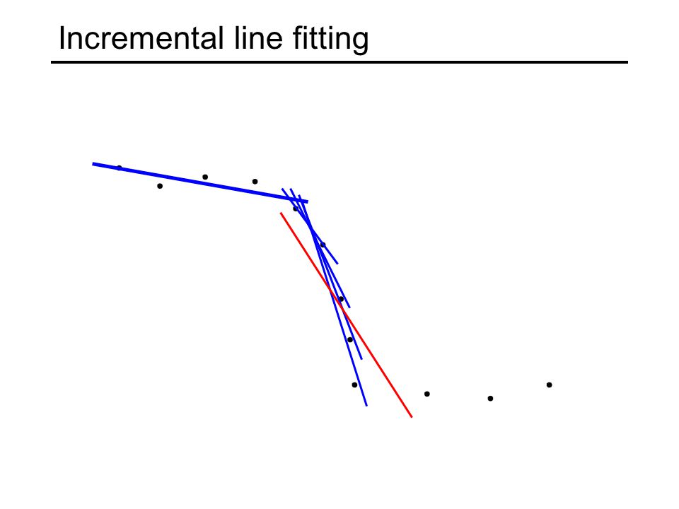
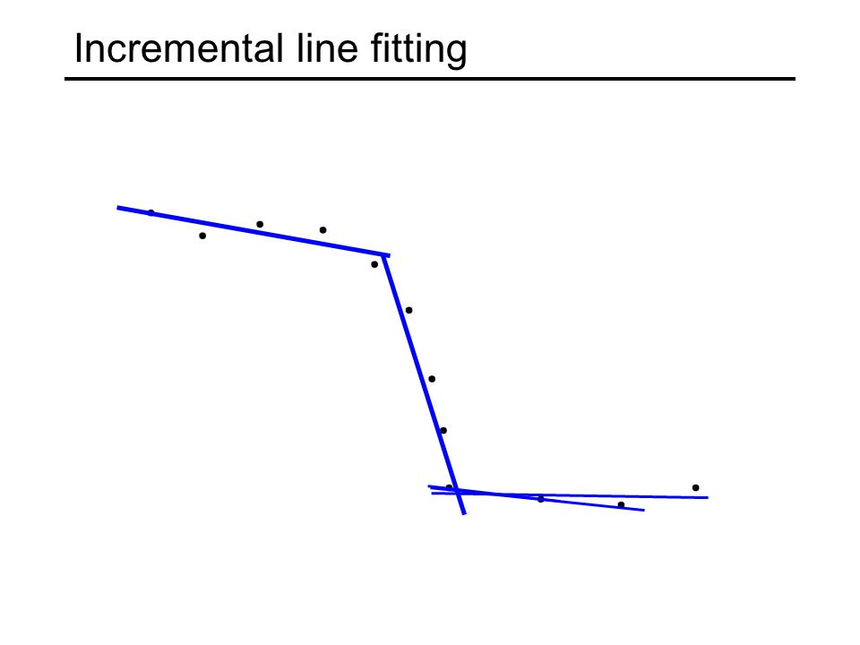
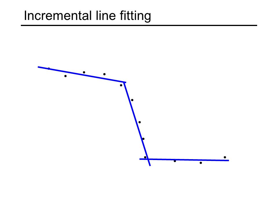
37. Incremental line fitting Examine edge points in their order along an edge chain Fit line to the first s points While line fitting residual is small enough, continue adding points to the current line and refitting When residual exceeds a threshold, break off current line and start a new one with the next s “unassigned” points

38. Incremental line fitting

42. Incremental fitting pros and cons Pros Exploits locality Adaptively determines the number of lines Cons Needs sequential ordering of features Can’t cope with occlusion Sensitive to noise and choice of threshold

43. Last time: Fitting Fitting without outliers: least squares Probabilistic interpretation Least squares for general curves Dealing with outliers Robust fitting RANSAC Fitting multiple lines Voting methods: Hough transform, RANSAC Incremental line fitting Next: K-lines

44. K-Lines Initialize k lines Option 1: Randomly initialize k sets of parameters Option 2: Randomly partition points into k sets and fit lines to them Iterate until convergence: Assign each point to the nearest line Refit parameters for each line

45. K-Lines example 1 initialization

46. K-Lines example 1 iteration 1: assignment to nearest line

47. K-Lines example 1 iteration 1: refitting

48. K-Lines example 2 initialization

49. iteration 1: assignment to nearest line K-Lines example 2

50. iteration 1: refitting

51. K-Lines example 2 iteration 2: assignment to nearest line

52. K-Lines example 2 iteration 2: refitting

53. K-Lines example 3 initialization

54. K-Lines example 3 iteration 2: assignment to nearest line

55. K-Lines example 3 iteration 1: refitting

56. K-Lines pros and cons Pros Guaranteed to reduce line fitting residual at each iteration Can cope with occlusion Cons Need to know k Can get stuck in local minima Sensitive to initialization

57. Expectation Maximization (EM) A more general probabilistic method for maximizing likelihood in the presence of missing data (i.e., assignments of points to lines)

58. Expectation Maximization (EM) We want to maximize the likelihood of the data points given parameters θ = {a k, b k, d k } of our lines:

59. Expectation Maximization (EM) We want to maximize the likelihood of the data points given parameters θ = {a k, b k, d k } of our lines: Missing data: assignment of points i to lines l k Iterate: Guess missing data using current model parameters Form maximum likelihood estimate of parameters using filled-in values for missing data Technical detail: need to take the expectation with respect to the distribution of the missing data The resulting procedure is guaranteed to increase likelihood at every iteration More on this later in the course (hopefully)

60. Application to recognition (teaser) Unsupervised learning: the target object is not segmented in the training image M. Weber, M. Welling and P. Perona, Unsupervised learning of models for recognition, ECCV 2000Unsupervised learning of models for recognition

61. Application to recognition (teaser) Unsupervised learning: the target object is not segmented in the training image M. Weber, M. Welling and P. Perona, Unsupervised learning of models for recognition, ECCV 2000Unsupervised learning of models for recognition Missing data: Face (eye, nose, mouth)? Background?

62. Task:Estimation of model parameters Let the assignments be a hidden variable and use EM algorithm to learn them and the model parameters Chicken and Egg type problem, since we initially know neither: - Model parameters - Assignment of regions to parts Slide credit: R. Fergus Learning using EM

63. E-step:Compute assignments for which regions belong to which part M-step:Update model parameters Find regions & their location & appearance Initialize model parameters Use EM and iterate to convergence: Trying to maximize likelihood – consistency in shape & appearance Slide credit: R. Fergus Learning procedure

64. Should we prefer a simpler or a more complex model? Two issues Which model fits the observed data best? Generalization performance: how well will a model predict points we haven’t seen before? Model selection

65. Bias-variance tradeoff Models with too many parameters may fit a given sample better, but have high variance Generalization error is due to overfitting Models with too few parameters may not fit a given sample well because of high bias Generalization error is due to underfitting 2

66. Given several models that describe the data equally well, the simpler one should be preferred There should be some tradeoff between error and model complexity This is rarely done rigorously, but is a powerful “rule of thumb” Simpler models are often preferred because of their robustness (= low variance) Occam’s razor

67. Review of key concepts Least squares fitting Probabilistic fitting The likelihood function Estimates: maximum likelihood, MAP Dealing with outliers Robust fitting RANSAC Fitting multiple lines Incremental fitting Voting: Hough transform, RANSAC Alternating minimization with “missing data”: K-lines, EM Model selection Bias vs. variance Occam’s razor