1. 3-D Large Eddy Simulation for Jet Noise Prediction A.Uzun, G. Blaisdell, A. Lyrintzis School of Aeronautics and Astronautics Purdue University Funded by the Indiana 21 st Century Research and Technology Fund

2. Motivation Aircraft noise regulations are becoming stricter Jet exhaust noise is the MAJOR component of aircraft engine noise at takeoff Need reliable jet noise prediction tools to aid in the design process of quiet engines

3. Objective Development and full validation of a Computational Aeroacoustics (CAA) methodology for jet noise prediction using:  A 3-D Large Eddy Simulation (LES) code working on generalized curvilinear grids that provides time-accurate unsteady flow field data  Integral acoustics methods coupled with LES data for far-field noise computations

5. Numerical Methods for LES 3-D filtered Navier-Stokes equations 6 th -order accurate compact differencing scheme for spatial derivatives 6 th -order spatial filtering for eliminating instabilities from unresolved scales and mesh non-uniformities 4 th -order Runge-Kutta time integration Localized dynamic Smagorinsky subgrid-scale (SGS) model for unresolved length scales Vortex ring forcing to trigger the instabilities

7. Code Parallelization Message Passing Interface (MPI) routines are used in the parallelization Compact difference scheme and the spatial filter both require solution of a system of equations along grid lines Parallelization is based on data transposition strategy

10. Computational Jet Noise Research State-of-the-art jet noise computations:  Freund’s DNS for Re D = 3600, Mach 0.9 cold jet using 25.6 million grid points (1999)  Bogey and Bailly’s LES for Re D = 400,000, Mach 0.9 isothermal jet using 12.5 and 16.6 million grid points (2002, 2003) We studied Mach 0.9 turbulent isothermal jets at Reynolds numbers of 100,000 and 400,000 12 million points used in Re D = 100,000 LES 15.6 million points used in Re D = 400,000 LES

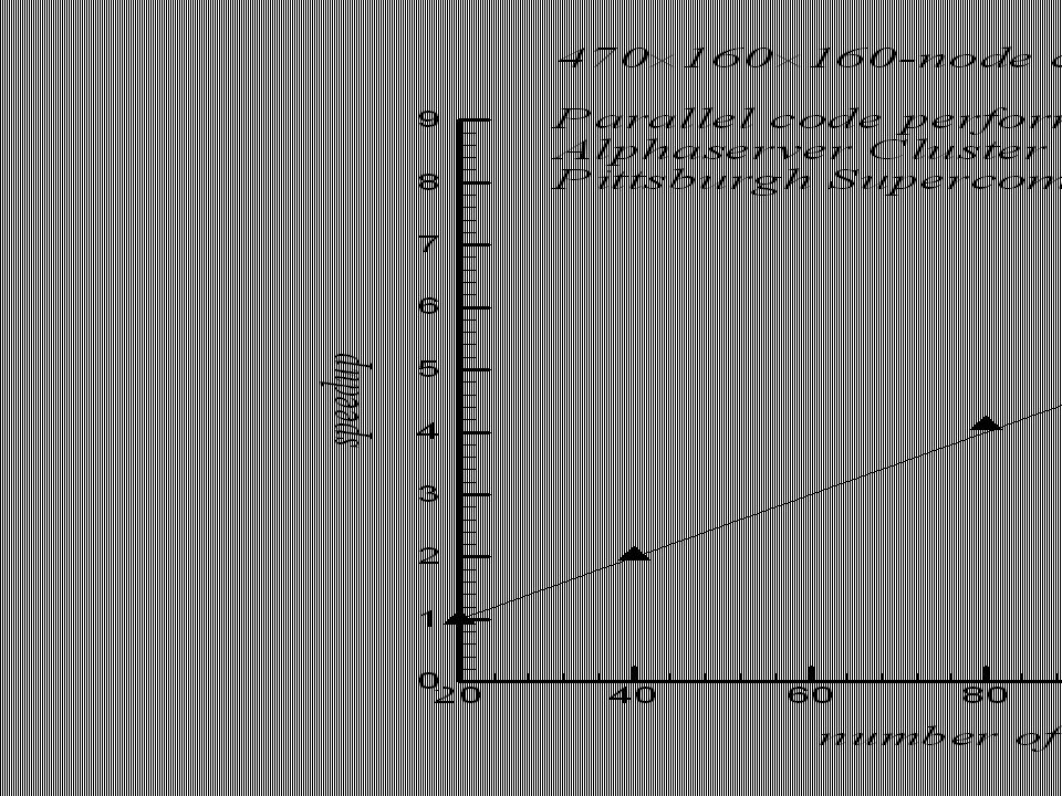
11. Computation Details (Re-100,000) Physical domain length of 60r o in streamwise direction Domain width and height are 40r o 470x160x160 (12 million) grid points Coarsest grid resolution: 170 times the local Kolmogorov length scale One month of run time on an IBM-SP using 160 processors to run 170,000 time steps Can do the same simulation on the Compaq Alphaserver Cluster at Pittsburgh Supercomputing Center in 10 days

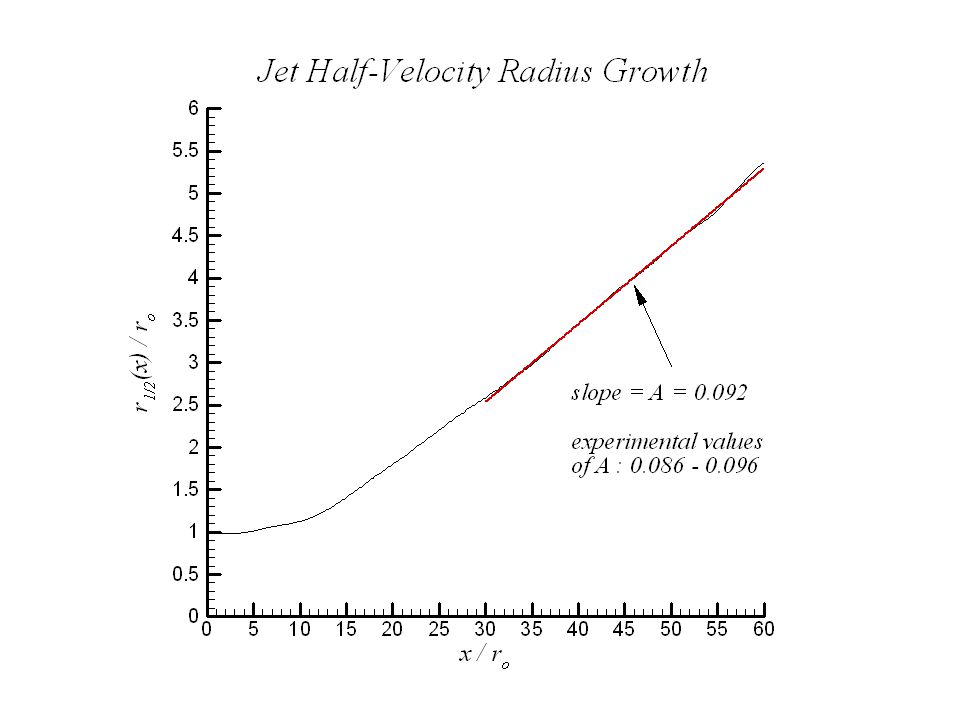
16. Mean Flow Results Our mean flow results are compared with:  Experiments of Zaman for initially compressible jets (1998)  Experiment of Hussein et al. (1994) Incompressible round jet at Re D = 95,500  Experiment of Panchapakesan et al. (1993) Incompressible round jet at Re D = 11,000

24. Jet Aeroacoustics Noise sources located at the end of potential core Far field noise is estimated by coupling near field LES data with the Ffowcs Williams–Hawkings (FWH) method Overall sound pressure level values are computed along an arc located at 60r o from the jet nozzle Cut-off Strouhal number based on grid resolution is around 1.0

27. OASPL results are compared with:  Experiment of Mollo-Christensen et al. (1964) Mach 0.9 round jet at Re D = 540,000 (cold jet)  Experiment of Lush (1971) Mach 0.88 round jet at Re D = 500,000 (cold jet)  Experiment of Stromberg et al. (1980) Mach 0.9 round jet at Re D =3,600 (cold jet)  SAE ARP 876C database Jet Aeroacoustics (continued)

29. Mach 0.9, Reynolds Number 400,000 Isothermal Jet LES No explicit SGS model Spatial filter is treated as the implicit SGS model 15.6 million grid points Streamwise physical domain length is 35r o Domain width and height are set to 30r o 50,000 time steps total 5.5 days of run time using 200 POWER3 processors on an IBM-SP3

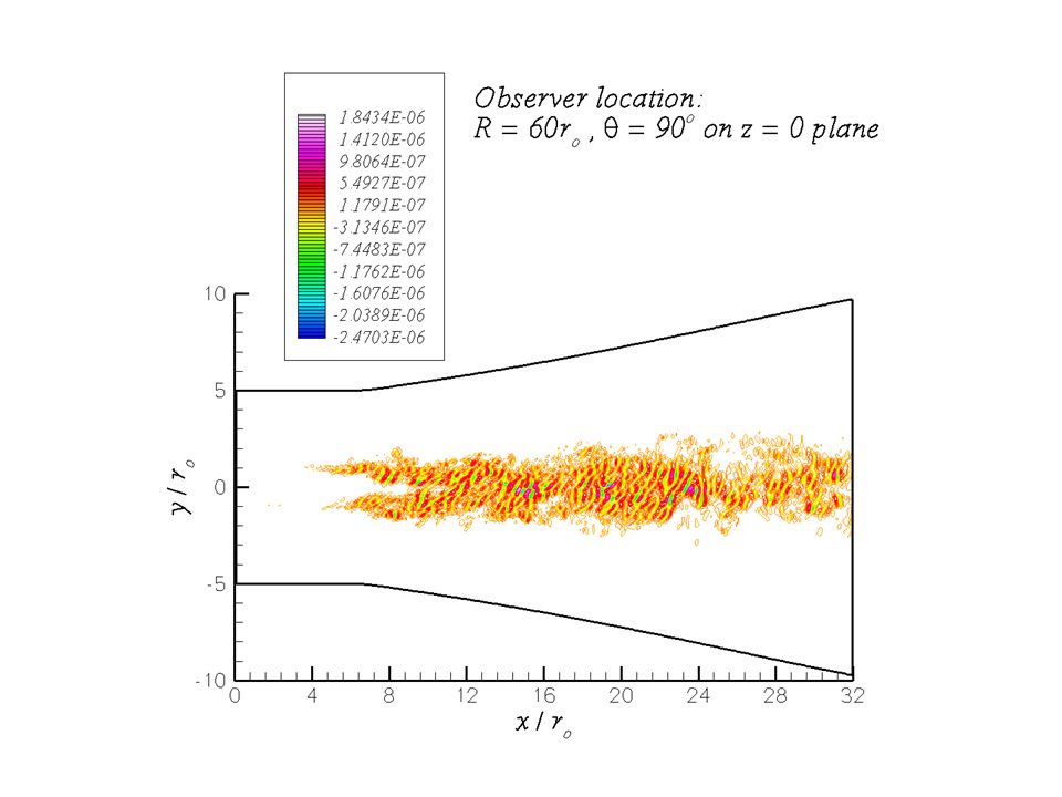
30. Divergence of Velocity Contours

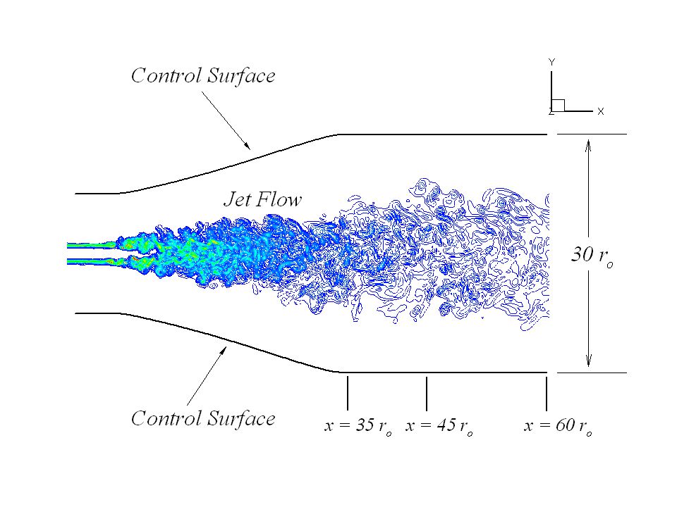
31. Jet Aeroacoustics (continued) Acoustic data collected every 5 time steps over a period of 25,000 time steps Shallow angles ( ) are not accurately captured since streamwise control surface is relatively short Maximum Strouhal numbers resolved (based on grid spacing) :  3.0 for Control Surface #1  2.0 for Control Surface #2  1.5 for Control Surface #3

32. Ffowcs Williams – Hawkings Method Prediction of Acoustic Pressure Spectra

33. Kirchhoff’s Method Prediction of Acoustic Pressure Spectra

34. Ffowcs Williams – Hawkings Method Prediction of OASPL

35. Kirchhoff’s Method Prediction of OASPL

36. Acoustic Pressure Spectra Comparison with Bogey and Bailly’s Reynolds number 400,000 LES

38. Closed Control Surface Calculations The control surface is closed on the outflow side Only the FW-H method is used with the closed control surface No refraction corrections employed

39. OASPL Comparison

40. Spectra Comparison at R = 60r o,  = 30 o

41. Noise Calculations Using Lighthill’s Acoustic Analogy Recently developed a parallel code which integrates Lighthill’s source term over a turbulent volume to compute far-field noise The code has the capability to compute the noise from the individual components of the Lighthill stress tensor

42. Lighthill Code Code employs the time derivative formulation of Lighthill’s volume integral Uses the time history of the jet flow data provided by the 3-D LES code 8 th -order accurate explicit scheme to compute the time derivatives Cubic spline interpolation to evaluate the source term at retarded times

43. Far-field Noise Time accurate data was saved inside the jet at every 10 time steps over a period of 40,000 time steps 1.2 Terabytes (TB) of total data to process Used 1160 processors in parallel for the volume integrals Cut-off frequency corresponds to Strouhal number 4.0 due to the fine grid spacing inside the jet

44. OASPL Predictions Using Lighthill Analogy

45. Animation #1 Animation on the next slide shows the time variation of the Lighthill sources that radiate noise in the direction of the observer located at R = 60r o,  = 30 o on the far-field arc

47. Animation #2 Animation on the next slide shows the time variation of the Lighthill sources that radiate noise in the direction of the observer located at R = 60r o,  = 90 o on the far-field arc

49. Acoustics Conclusions Both FW–H and Kirchhoff’s methods give almost identical results for all open control surfaces Closed control surface + FW-H give predictions comparable to Lighthill’s acoustic analogy prediction Due to the inflow forcing, OASPL levels are overpredicted relative to experiments There are acoustic sources (causing cancellations) located in the region 32r o < x which were not captured in the LES due to short domain size

50. Conclusions Localized dynamic SGS and implicit SGS models are stable and robust for the jet flows studied Very good comparison of mean flow results with experiments Aeroacoustics results are encouraging

51. Future Directions Noise from unresolved LES scales: - Resolved Scales: LES + FW-H - Unresolved Scales: MGB/Tam’s approach (as currently used for RANS) Include nozzle lips Complicated geometries (DES for chevrons, mixers -- multi-block code) Supersonic jets