1. (Z&B) Steps in Transport Modeling Calibration step (calibrate flow model & transport model) Adjust parameter values

2. Input Parameters for Transport Simulation Flow Transport hydraulic conductivity (K x, K y K z ) storage coefficient (S s, S, S y ) porosity (  ) dispersivity (  L,  TH,  TV ) retardation factor or distribution coefficient 1 st order decay coefficient or half life recharge rate pumping rates source term (mass flux) All of these parameters potentially could be estimated during calibration. That is, they are potentially calibration parameters.

3. Comparison of measured and simulated concentrations

4. A GWV calibration plot Observed value Model Value Perfect match

5. Average calibration errors (residuals) are reported as: Mean Absolute Error (MAE) = 1/N   calculated i – observed i  Root Mean Squared Error (RMS) =  1/N  (calculated i – observed i ) 2  ½ Sum of squared residuals =  (calculated i – observed i ) 2

6. Example listing of residuals in head targets in GWV

7. Calibration of a flow model is generally straightforward: Match model results to an observed steady state flow field If possible, verify with a transient calibration Calibration to flow is non-unique. Calibration of a transport model is more difficult: There are more potential calibration parameters There is greater potential for numerical error in the solution The measured concentration data needed for calibration may be sparse or non-existent Transport calibrations are non-unique.

8. Borden Plume Simulated: double-peaked source concentration (best calibration) Simulated: smooth source concentration (best calibration) Z&B, Ch. 14 Calibration is non-unique. Two sets of parameter values give equally good matches to the observed plume.

9. “Trial and error” method of calibration Assumed source input function R=1 R=3 R=6 observed

10. Modeling done by Maura Metheny for the PhD under the direction of Prof. Scott Bair, Ohio State University Case Study: Woburn, Massachusetts TCE (Trichloroethene)

11. Common organic contaminants Source: EPA circular

12. Spitz and Moreno (1996) fraction of organic carbon

13. Spitz and Moreno ( 1996)

14. 01000 feet TCE in 1985 W.R. Grace Beatrice Foods Woburn Site Municipal Wells G & H Aberjona River Geology: buried river valley of glacial outwash and ice contact deposits overlying fractured bedrock The trial took place in 1986. Did TCE reach the wells before May 1979? Wells G&H operated from October 1964- May 1979

15. MODFLOW, MT3D, and GWV 6 layers, 93 rows, 107 columns (30,111 active cells) Woburn Model: Design The transport model typically took two to three days to run on a 1.8 gigahertz PC with 1024K MB RAM. Wells operated from October 1964- May 1979 Simulation run from Jan. 1960 to Dec. 1985 using 55 stress periods (to account for changes in pumping and recharge owing to changes in precipitation and land use) Five sources of TCE were included in the model: New England Plastics Wildwood Conservation Trust (Riley Tannery/Beatrice Foods) Olympia Nominee Trust (Hemingway Trucking) UniFirst W.R. Grace (Cryovac)

16. (Z&B) Steps in Transport Modeling Calibration step (calibrate flow model & transport model) Adjust parameter values

17. Calibration of a flow model is generally straightforward: Match model results to an observed steady state flow field If possible, verify with a transient calibration Calibration to flow is non-unique. Calibration of a transport model is more difficult: There are more potential calibration parameters There is greater potential for numerical error in the solution The measured concentration data needed for calibration may be sparse or non-existent Transport calibrations are non-unique. Calibration Targets: concentrations Calibration Targets: Heads and fluxes

18. Source term input function From Zheng and Bennett Used as a calibration parameter in the Woburn model Other possible calibration parameters include: K, recharge, boundary conditions dispersivities chemical reaction terms

19. Flow model (included heterogeneity in K, S and  ) Water levels Streamflow measurements Groundwater velocities from helium/tritium groundwater ages It cannot be determined which, if any, of the plausible scenarios actually represents what occurred in the groundwater flow system during this period, even though each of the plausible scenarios closely reproduces measured values of TCE. Woburn Model: Calibration Transport Model (included retardation) The animation represents one of several equally plausible simulations of TCE transport based on estimates of source locations, source concentrations, release times, and retardation. The group of plausible scenarios was developed because the exact nature of the TCE sources is not precisely known. A trial and error calibration

20. Automated Calibration From Zheng and Bennett Codes: UCODE, PEST, MODFLOWP Case Study

21. From Zheng and Bennett source term Sum of squared residuals =  (calculated i – observed i ) 2 Transport data are useful in calibrating a flow model recharge

22. Comparison of observed vs. simulated concentrations at 3 wells for the 10 parameter simulation. From Zheng and Bennett

23. Sensitivity Coefficients p. 343, Z&B Sensitivity Analysis

24. Example of a sensitivity analysis of a flow model From Zheng and Bennett

25. Normalized sensitivity coefficient of travel time with respect to hydraulic conductivity

26. TMR (telescopic mesh refinement) From Zheng and Bennett TMR is used to cut out and define boundary conditions around a local area within a regional flow model.

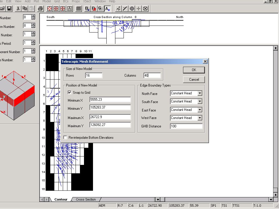
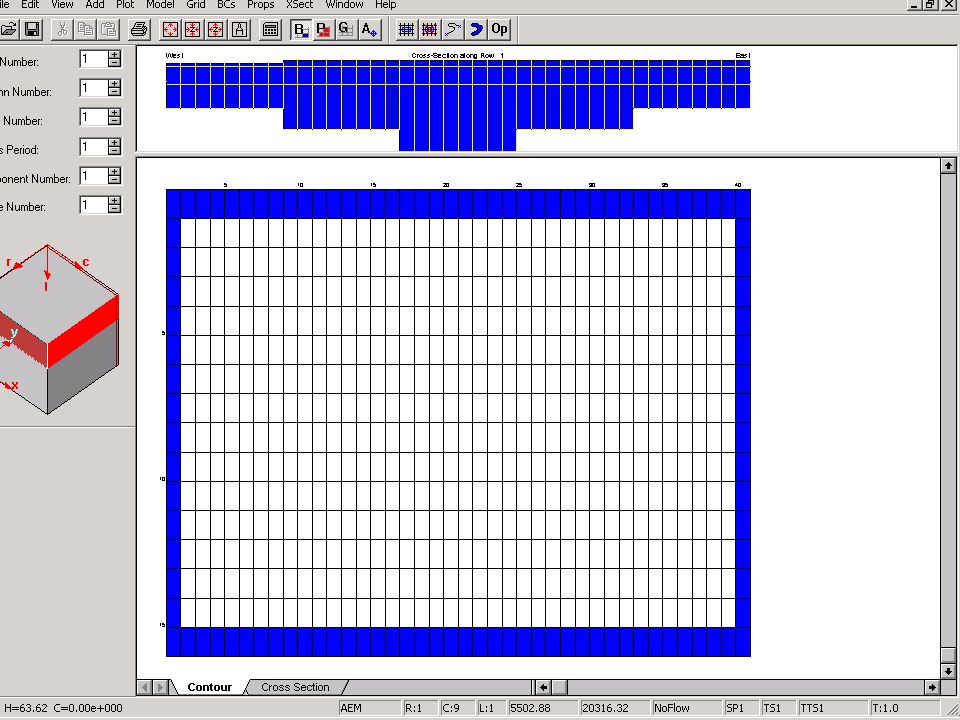
27. GWV option for Telescopic Mesh Refinement (TMR)

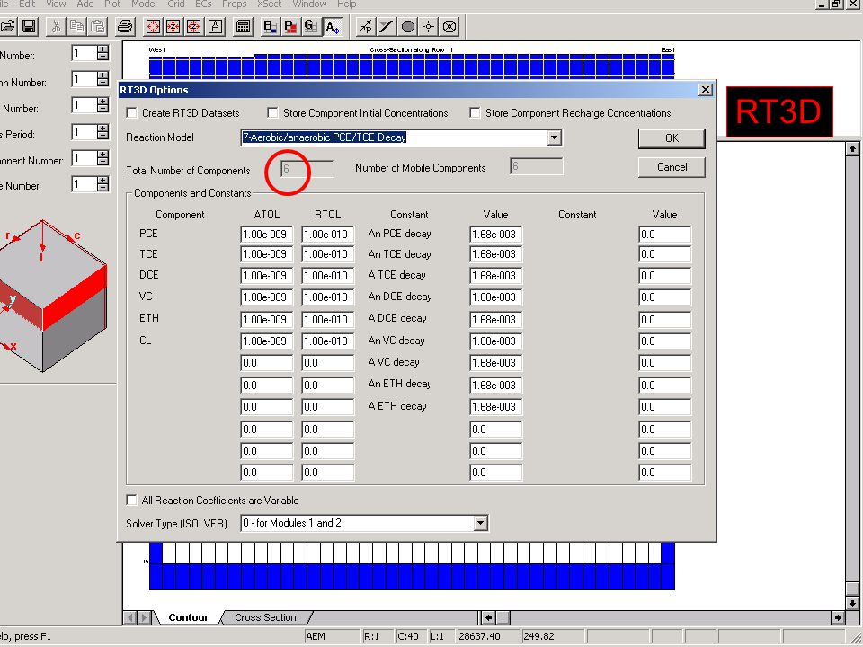
30. Multiple Species – MT3DMS RT3D