1. Forecasting using simple models

2. Outline Basic forecasting models The basic ideas behind each model
When each model may be appropriate
Illustrate with examples
Forecast error measures
Automatic model selection
Adaptive smoothing methods
(automatic alpha adaptation)
Ideas in model based forecasting techniques
Regression
Autocorrelation
Prediction intervals

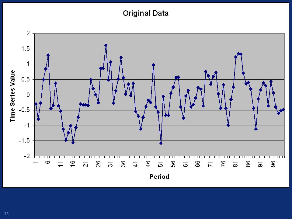
3. Basic Forecasting Models
Moving average and weighted moving average
First order exponential smoothing
Second order exponential smoothing
First order exponential smoothing with trends and/or seasonal patterns
Croston’s method

4. M-Period Moving Average
i.e. the average of the last M data points
Basically assumes a stable (trend free) series
How should we choose M?
Advantages of large M?
Average age of data = M/2

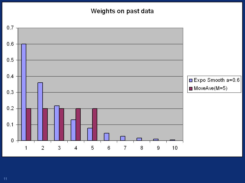
5. Weighted Moving Averages
The Wi are weights attached to each historical data point
Essentially all known (univariate) forecasting schemes are weighted moving averages
Thus, don’t screw around with the general versions unless you are an expert

6. Simple Exponential Smoothing
Pt+1(t) = Forecast for time t+1 made at time t
Vt = Actual outcome at time t
0<<1 is the “smoothing parameter”

7. Two Views of Same Equation
Pt+1(t) = Pt(t-1) + [Vt – Pt(t-1)]
Adjust forecast based on last forecast error OR
Pt+1(t) = (1- )Pt(t-1) + Vt
Weighted average of last forecast and last Actual

8. Simple Exponential Smoothing
Is appropriate when the underlying time series behaves like a constant + Noise
Xt =  + Nt
Or when the mean  is wandering around
That is, for a quite stable process
Not appropriate when trends or seasonality present

9. ES would work well here

10. Simple Exponential Smoothing
We can show by recursive substitution that ES can also be written as:
Pt+1(t) = Vt + (1-)Vt-1 + (1-)2Vt-2 + (1-)3Vt-3 +…..
Is a weighted average of past observations
Weights decay geometrically as we go backwards in time

12. Simple Exponential Smoothing
Ft+1(t) = At + (1-)At-1 + (1-)2At-2 + (1-)3At-3 +…..
Large  adjusts more quickly to changes
Smaller  provides more “averaging” and thus lower variance when things are stable
Exponential smoothing is intuitively more appealing than moving averages

13. Exponential Smoothing Examples

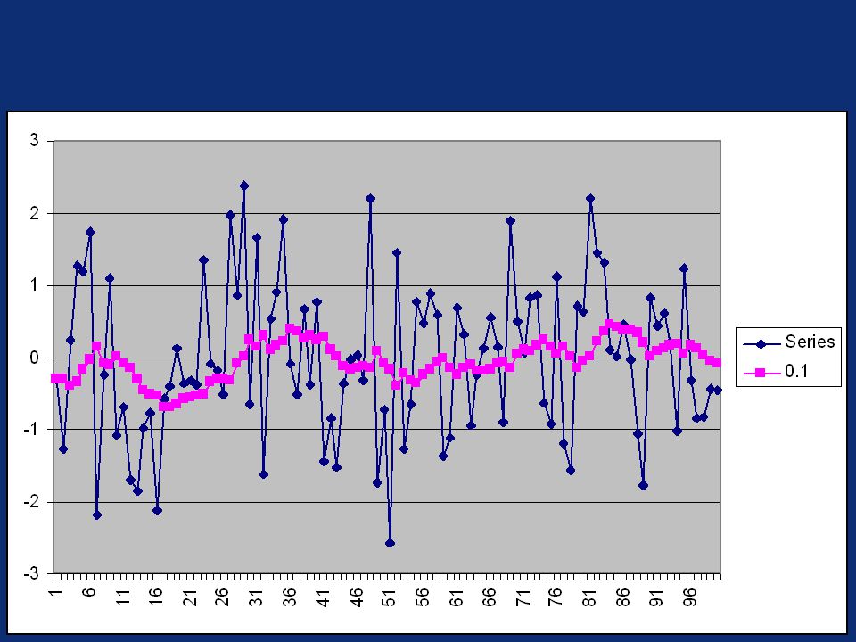
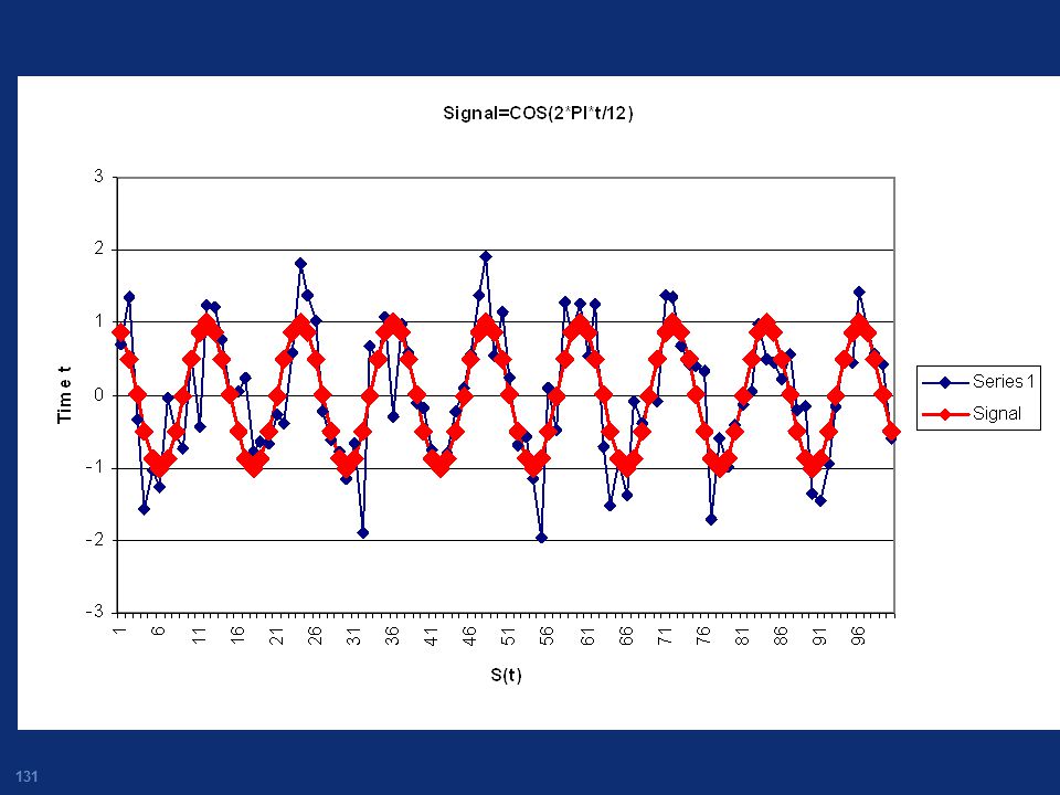
14. Zero Mean White Noise

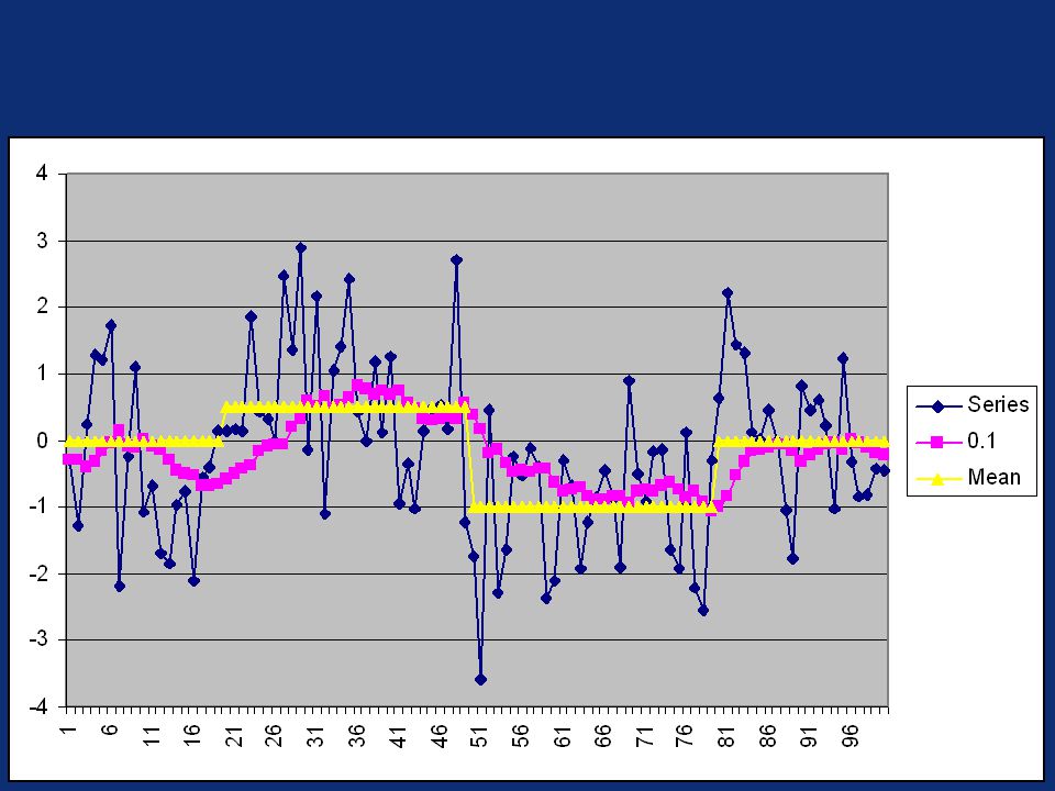
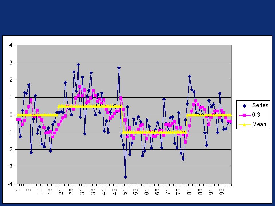
17. Shifting Mean + Zero Mean White Noise

20. Automatic selection of 
Using historical data
Apply a range of  values
For each, calculate the error in one-step-ahead forecasts
e.g. the root mean squared error (RMSE)
Select the  that minimizes RMSE

21. RMSE vs Alpha
1.45
1.4
1.35
RMSE
1.3
1.25
1.2
1.15
0.1
0.2
0.3
0.4
0.5
0.6
0.7
0.8
0.9 1
Alpha

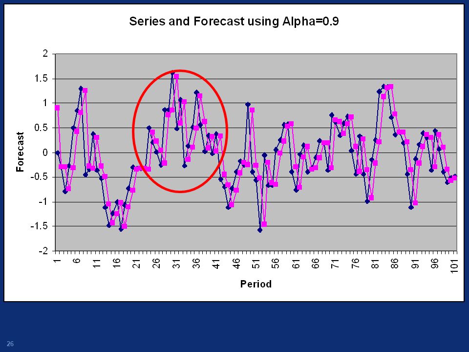
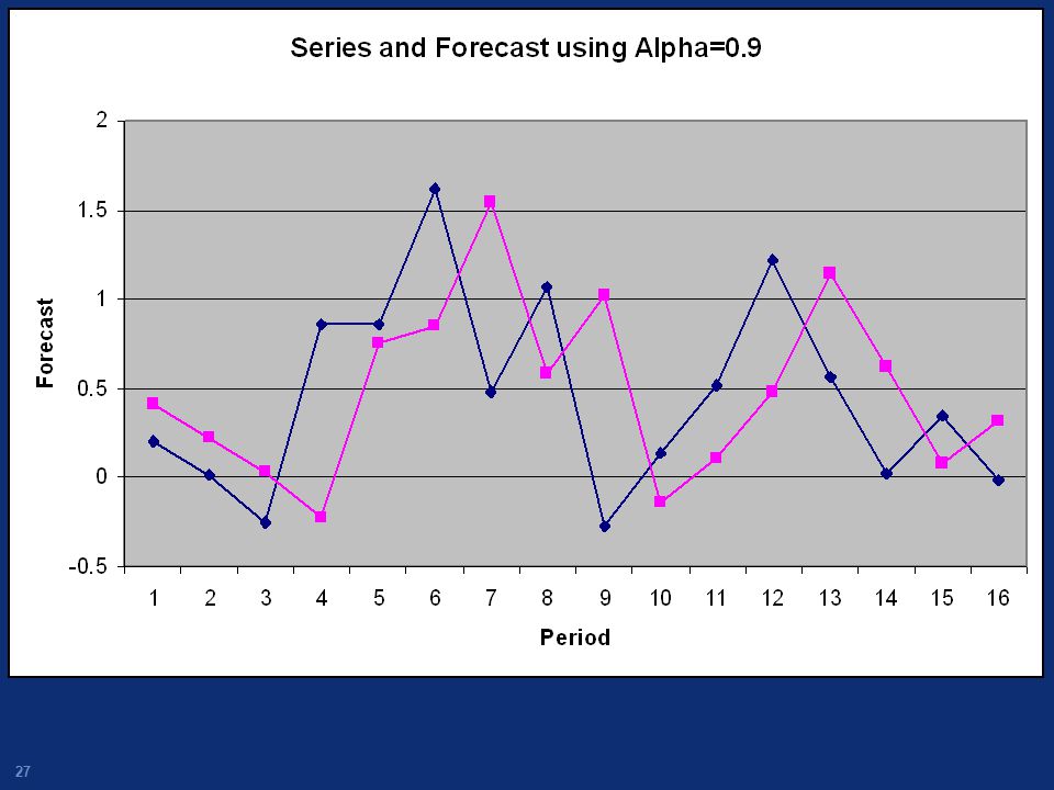
22. Recommended Alpha Typically alpha should be in the range 0.05 to 0.3
If RMSE analysis indicates larger alpha, exponential smoothing may not be appropriate

25. Might look good, but is it?

28. Series and Forecast using Alpha=0.92
1.5 1
Forecast
0.5
-0.5 1 2 3 4 5 6 7 8 9 10 11 12 13 14 15 16
Period

29. Forecast RMSE vs Alpha 0.67 0.66 0.65 0.64 0.63 Forecast RMSE 0.62
Series1
0.61
0.6
0.59
0.58
0.57
0.2
0.4
0.6
0.8 1
Alpha

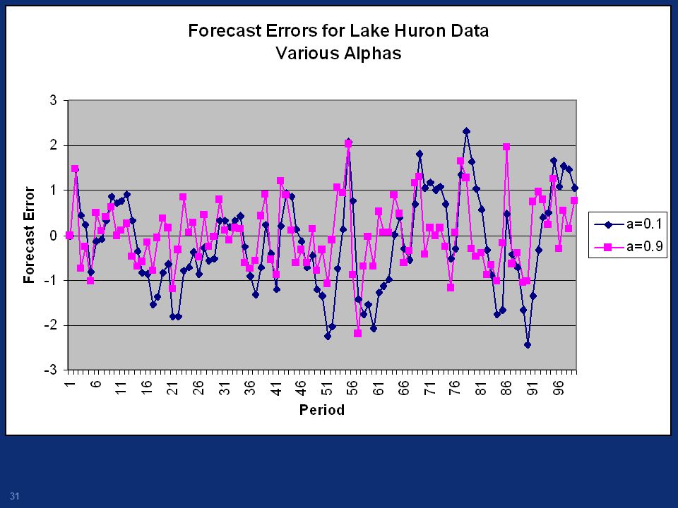
32. Forecast RMSE vs Alpha for Lake Huron Data
1.1
1.05 1
0.95
0.9
RMSE
0.85
0.8
0.75
0.7
0.65
0.6
0.1
0.2
0.3
0.4
0.5
0.6
0.7
0.8
0.9 1
Alpha

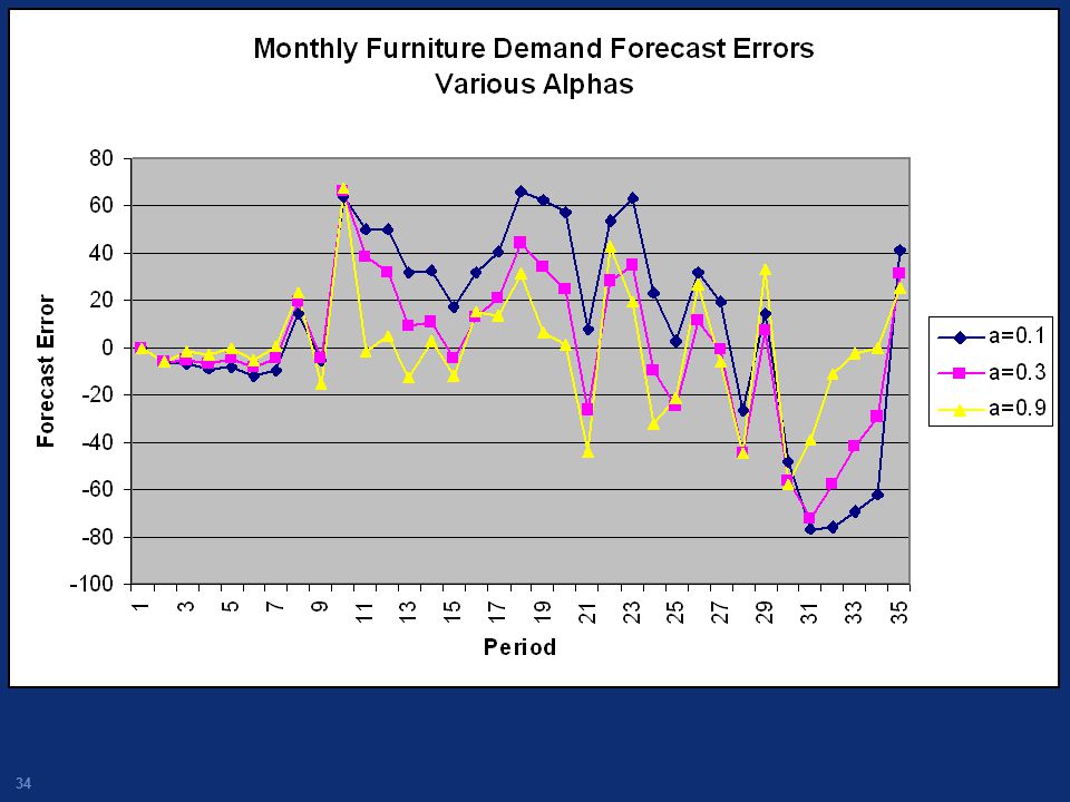
35. for Monthly Furniture Demand Data
Forecast RMSE vs Alpha
for Monthly Furniture Demand Data
45.6
40.6
35.6
30.6
25.6
RMSE
20.6
15.6
10.6
5.6
0.6
0.1
0.2
0.3
0.4
0.5
0.6
0.7
0.8
0.9 1
Alpha

36. Exponential smoothing will lag behind a trend
Suppose Xt=b0+ b1t
And St= (1- )St-1 + Xt
Can show that

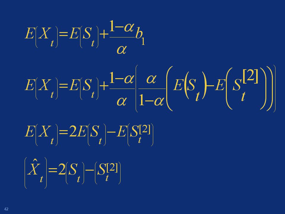
38. Double Exponential Smoothing
Modifies exponential smoothing for following a linear trend
i.e. Smooth the smoothed value

39. St Lags
St[2] Lags even more

40. 2St -St[2] doesn’t lag

44. Example

45. =0.2

46. Single Lags a trend

47. Double Over-shoots a change (must “re-learn” the slope)6 5 4
Double Over-shoots a change
(must “re-learn” the slope) 3
Trend 2
Series Data
Single Smoothing 1
Double smoothing -1 1 6 11 16 21 26 31 36 41 46 51 56 61 66 71 76 81 86 91 96
101

48. Holt-Winters Trend and Seasonal Methods
“Exponential smoothing for data with trend and/or seasonality”
Two models, Multiplicative and Additive
Models contain estimates of trend and seasonal components
Models “smooth”, i.e. place greater weight on more recent data

49. Winters Multiplicative Model
Xt = (b1+b2t)ct + t
Where ct are seasonal terms and
Note that the amplitude depends on the level of the series
Once we start smoothing, the seasonal components may not add to L

50. Holt-Winters Trend Model
Xt = (b1+b2t) + t
Same except no seasonal effect
Works the same as the trend + season model except simpler

51. Example:

52. (1+0.04t)

53. *150%

54. *50%

55. The seasonal terms average 100% (i.e. 1)
Thus summed over a season, the ct must add to L
Each period we go up or down some percentage of the current level value
The amplitude increasing with level seems to occur frequently in practice

56. Recall Australian Red Wine Sales

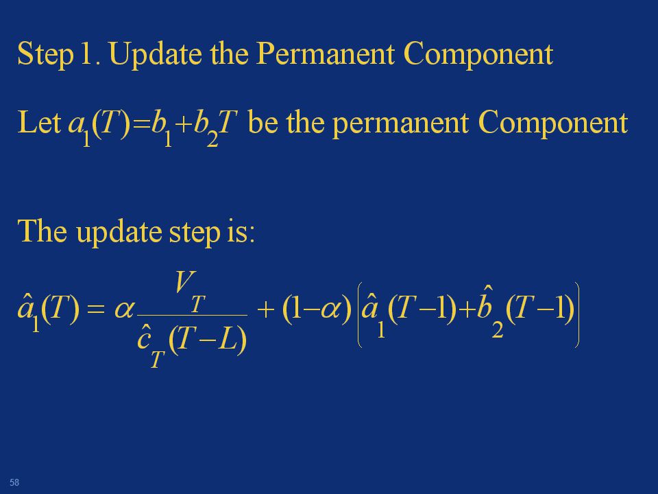
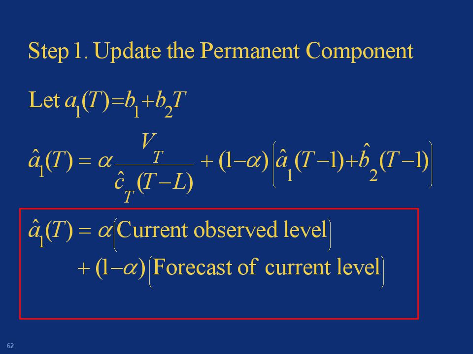
57. Smoothing
In Winters model, we smooth the “permanent component”, the “trend component” and the “seasonal component”
We may have a different smoothing parameter for each (, , )
Think of the permanent component as the current level of the series (without trend)

59. Current Observation

60. Current Observation
“deseasonalized”

61. Estimate of permanent component from
last time = last level + slope*1

64. “observed” slope

65. “observed” slope
“previous” slope

68. Extend the trend out  periods ahead

69. Use the proper seasonal adjustment

70. Winters Additive Method
Xt = b1+ b2t + ct + t
Where ct are seasonal terms and
Similar to previous model except we “smooth” estimates of b1, b2, and the ct

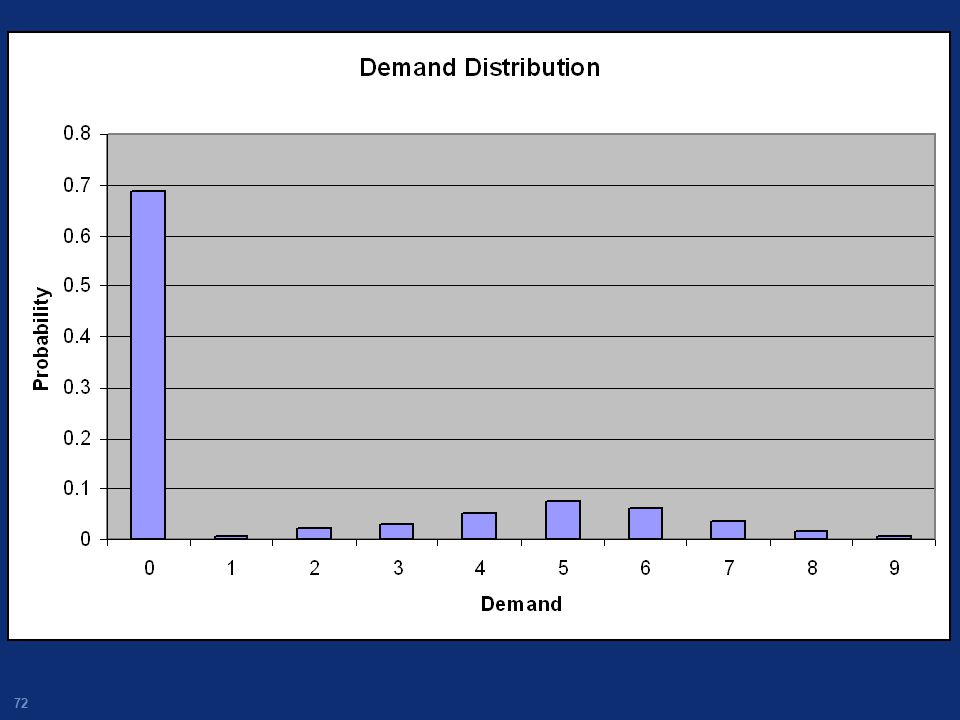
71. Croston’s Method
Can be useful for intermittent, erratic, or slow-moving demand
e.g. when demand is zero most of the time (say 2/3 of the time)
Might be caused by
Short forecasting intervals (e.g. daily)
A handful of customers that order periodically
Aggregation of demand elsewhere (e.g. reorder points)

73. Typical situation Central spare parts inventory (e.g. military)
Orders from manufacturer
in batches (e.g. EOQ)
periodically when inventory nearly depleted
long lead times may also effect batch size

74. Example
Demand each
period follows a
distribution that
is usually zero

75. Example

76. Example
Exponential smoothing applied (=0.2)

77. Using Exponential Smoothing:
Forecast is highest right after a non-zero demand occurs
Forecast is lowest right before a non-zero demand occurs

78. Croston’s Method Forecast = Separately Tracks
Time between (non-zero) demands
Demand size when not zero
Smoothes both time between and demand size
Combines both for forecasting
Demand Size
Forecast =
Time between demands

79. Define terms V(t) = actual demand outcome at time t
P(t) = Predicted demand at time t
Z(t) = Estimate of demand size (when it is not zero)
X(t) = Estimate of time between (non-zero) demands
q = a variable used to count number of periods between non-zero demand

80. Forecast Update For a period with zero demand Z(t)=Z(t-1) X(t)=X(t-1)
No new information about
order size Z(t)
time between orders X(t)
q=q+1
Keep counting time since last order

81. Forecast Update q=1 For a period with non-zero demand
Z(t)=Z(t-1) + (V(t)-Z(t-1))
X(t)=X(t-1) + (q - X(t-1))
q=1

82. Forecast Update q=1 Latest order size
For a period with non-zero demand
Z(t)=Z(t-1) + (V(t)-Z(t-1))
X(t)=X(t-1) + (q - X(t-1))
q=1
Update Size of order via smoothing
Latest
order size

83. Forecast Update q=1 Latest time between orders
For a period with non-zero demand
Z(t)=Z(t-1) + (V(t)-Z(t-1))
X(t)=X(t-1) + (q - X(t-1))
q=1
Update size of order via smoothing
Update time between orders via smoothing
Latest time
between orders

84. Forecast Update q=1 Reset counter For a period with non-zero demand
Z(t)=Z(t-1) + (V(t)-Z(t-1))
X(t)=X(t-1) + (q - X(t-1))
q=1
Update size of order via smoothing
Update time between orders via smoothing
Reset counter of time between orders
Reset
counter

85. Forecast P(t) = = Finally, our forecast is: Z(t) Non-zero Demand Size
X(t) Time Between Demands

86. Recall example
Exponential smoothing applied (=0.2)

87. Recall example
Croston’s method applied (=0.2)

88. True average demand per period=0.176
What is it forecasting?
Average demand per period
True average demand per period=0.176

89. Behavior Forecast only changes after a demand
Forecast constant between demands
Forecast increases when we observe
A large demand
A short time between demands
Forecast decreases when we observe
A small demand
A long time between demands

90. Croston’s Method
Croston’s method assumes demand is independent between periods
That is one period looks like the rest
(or changes slowly)

91. Counter Example One large customer Orders using a reorder point
The longer we go without an order
The greater the chances of receiving an order
In this case we would want the forecast to increase between orders
Croston’s method may not work too well

92. Better Examples Demand is a function of intermittent random events
Military spare parts depleted as a result of military actions
Umbrella stocks depleted as a function of rain
Demand depending on start of construction of large structure

93. Is demand Independent?
If enough data exists we can check the distribution of time between demand
Should “tail off” geometrically

94. Theoretical behavior

95. In our example:

96. Comparison

97. Counterexample
Croston’s method might not be appropriate if the time between demands distribution looks like this:

98. Counterexample
In this case, as time approaches 20 periods without demand, we know demand is coming soon.
Our forecast should increase in this case

99. Error Measures
Errors: The difference between actual and predicted (one period earlier)
et = Vt – Pt(t-1)
et =can be positive or negative
Absolute error |et|
Always positive
Squared Error et2
The percentage error PEt = 100et / Vt
Can be positive or negative

100. Bias and error magnitude
Forecasts can be:
Consistently too high or too low (bias)
Right on average, but with large deviations both positive and negative (error magnitude)
Should monitor both for changes

101. Error Measures Look at errors over time
Cumulative measures summed or averaged over all data
Error Total (ET)
Mean Percentage Error (MPE)
Mean Absolute Percentage Error (MAPE)
Mean Squared Error (MSE)
Root Mean Squared Error (RMSE)
Smoothed measures reflects errors in the recent past
Mean Absolute Deviation (MAD)

102. Error Measures Measure Bias Look at errors over time
Cumulative measures summed or averaged over all data
Error Total (ET)
Mean Percentage Error (MPE)
Mean Absolute Percentage Error (MAPE)
Mean Squared Error (MSE)
Root Mean Squared Error (RMSE)
Smoothed measures reflects errors in the recent past
Mean Absolute Deviation (MAD)

103. Error Measures Measure error magnitude Look at errors over time
Cumulative measures summed or averaged over all data
Error Total (ET)
Mean Percentage Error (MPE)
Mean Absolute Percentage Error (MAPE)
Mean Squared Error (MSE)
Root Mean Squared Error (RMSE)
Smoothed measures reflects errors in the recent past
Mean Absolute Deviation (MAD)

104. Error Total Sum of all errors Uses raw (positive or negative) errors
ET can be positive or negative
Measures bias in the forecast
Should stay close to zero as we saw in last presentation

105. MPE Average of percent errors Can be positive or negative
Measures bias, should stay close to zero

106. MSE Average of squared errors Always positive
Measures “magnitude” of errors
Units are “demand units squared”

107. RMSE Square root of MSE Always positive Measures “magnitude” of errors
Units are “demand units”
Standard deviation of forecast errors

108. MAPE Average of absolute percentage errors Always positive
Measures magnitude of errors
Units are “percentage”

109. Mean Absolute Deviation
Smoothed absolute errors
Always positive
Measures magnitude of errors
Looks at the recent past

110. Percentage or Actual units
Often errors naturally increase as the level of the series increases
Natural, thus no reason for alarm
If true, percentage based measured preferred
Actual units are more intuitive

111. Squared or Absolute Errors
Absolute errors are more intuitive
Standard deviation units less so
66% within  1 S.D.
95% within  2 S.D.
When using measures for automatic model selection, there are statistical reasons for preferring measures based on squared errors

112. Ex-Post Forecast Errors
Given
A forecasting method
Historical data
Calculate (some) error measure using the historical data
Some data required to initialize forecasting method.
Rest of data (if enough) used to calculate ex-post forecast errors and measure

113. Automatic Model Selection
For all possible forecasting methods
(and possibly for all parameter values e.g. smoothing constants – but not in SAP?)
Compute ex-post forecast error measure
Select method with smallest error

114. Automatic  Adaptation
Suppose an error measure indicates behavior has changed
e.g. level has jumped up
Slope of trend has changed
We would want to base forecasts on more recent data
Thus we would want a larger 

115. Tracking Signal (TS)
Bias/Magnitude = “Standardized bias”

116.  Adaptation If TS increases, bias is increasing, thus increase 
I don’t like these methods due to instability

117. Model Based Methods Find and exploit “patterns” in the data
Trend and Seasonal Decomposition
Time based regression
Time Series Methods (e.g. ARIMA Models)
Multiple Regression using leading indicators
Assumes series behavior stays the same
Requires analysis (no “automatic model generation”)

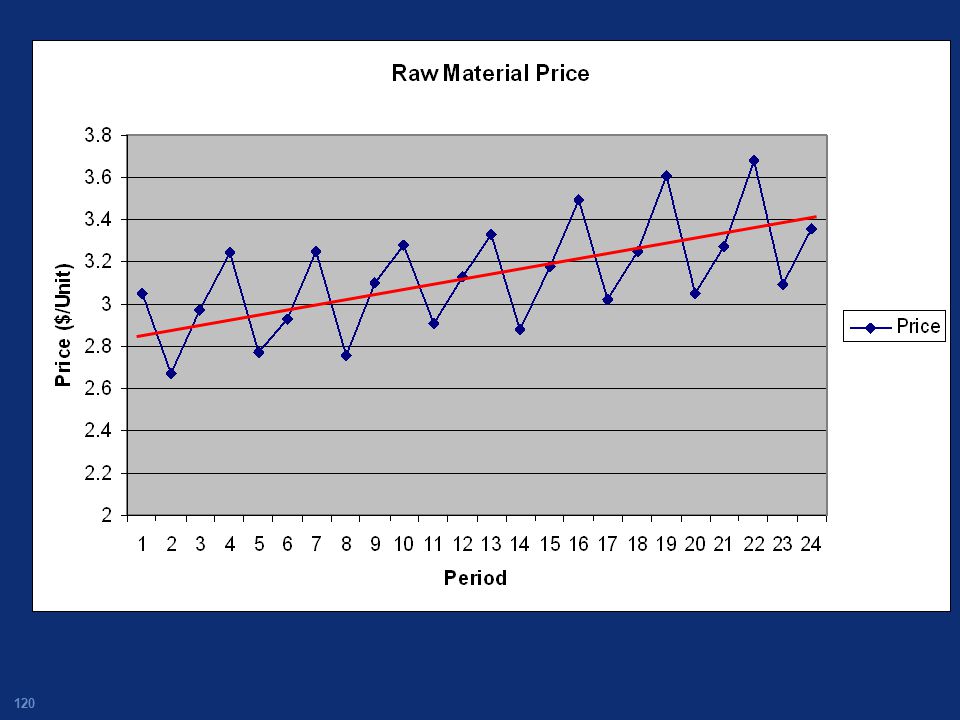
118. Univariate Time Series Models Based on Decomposition
Vt = the time series to forecast
Vt = Tt + St + Nt
Where
Tt is a deterministic trend component
St is a deterministic seasonal/periodic component
Nt is a random noise component

119. (Vt)=0.257

121. Simple Linear Regression Model: Vt=2.877174+0.020726t

122. Use Model to Forecast into the Future

123. Residuals = Actual-Predicted et = Vt-(2.877174+0.020726t)

124. Simple Seasonal Model
Estimate a seasonal adjustment factor for each period within the season
e.g. SSeptember

125. Sorted
by season
Season
averages

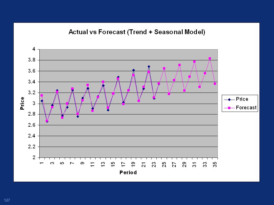
126. Trend + Seasonal Model Vt=2.877174+0.020726t + Smod(t,3) Where

128. et = Vt - ( t + Smod(t,3))
(et)=0.145

129. Can use other trend models
Vt= 0+ 1Sin(2t/k) (where k is period)
Vt= 0+ 1t + 2t2 (multiple regression)
Vt= 0+ 1ekt
etc.
Examine the plot, pick a reasonable model
Test model fit, revise if necessary

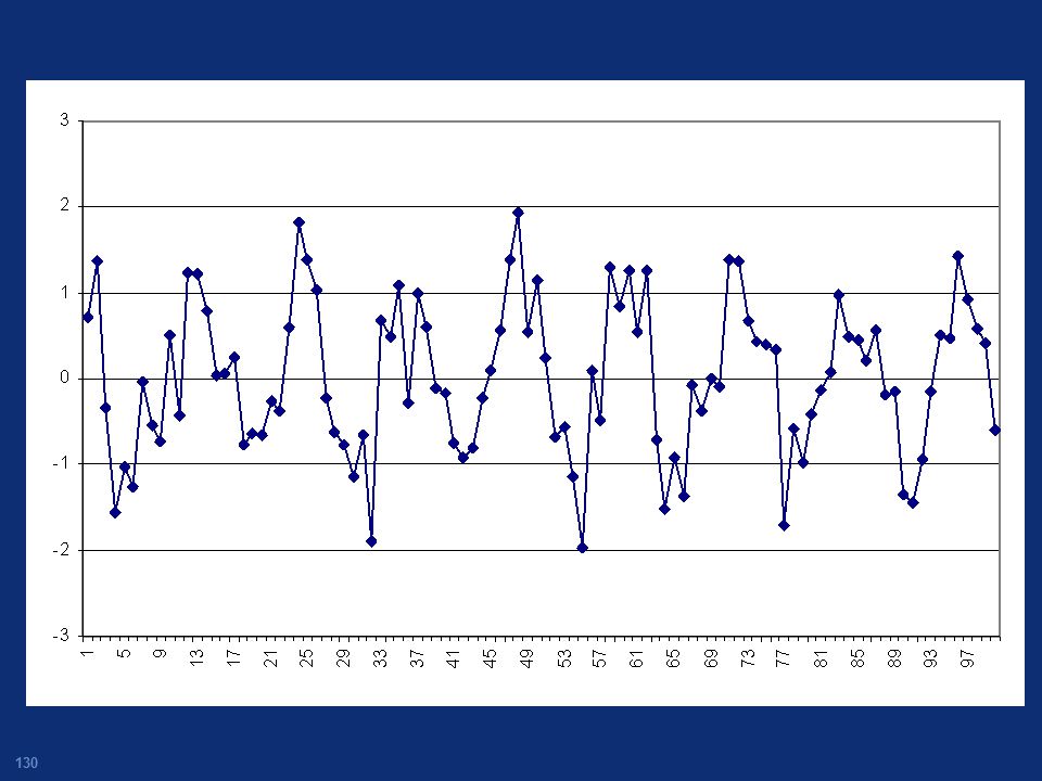
132. Model: Vt = Tt + St + Nt
After extracting trend and seasonal components we are left with “the Noise”
Nt = Vt – (Tt + St)
Can we extract any more predictable behavior from the “noise”?
Use Time Series analysis
Akin to signal processing in EE

133. Zero Mean, and Aperiodic: Is our best forecast ?

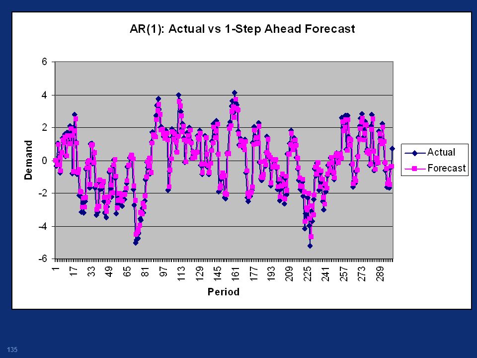
134. AR(1) Model This data was generated using the model Nt = 0.9Nt-1 + Zt
Where Zt ~N(0,2)
Thus to forecast Nt+1,we could use:

137. Time Series Models
Examine the correlation of the time series to past values.
This is called “autocorrelation”
If Nt is correlated to Nt-1, Nt-2,…..
Then we can forecast better than

138. Sample Autocorrelation Function

139. Back to our Demand Data

140. No Apparent Significant Autocorrelation

141. Multiple Linear Regression
V= 0+ 1 X1 + 2 X2 +….+ p Xp + 
Where
V is the “independent variable” you want to predict
The Xi‘s are the dependent variables you want to use for prediction (known)
Model is linear in the i‘s

142. Examples of MLR in Forecasting
Vt= 0+ 1t + 2t2 + 3Sin(2t/k) + 4ekt
i.e a trend model, a function of t
Vt= 0+ 1X1t + 2X2t
Where X1t and X2t are leading indicators
Vt= 0+ 1Vt-1+ 2Vt-2 + 12Vt-12 +13Vt-13
An Autoregressive model

143. Example: Sales and Leading Indicator

144. Example: Sales and Leading Indicator
Sales(t) = Sales(t-3)
-0.78Sales(t-2)+1.22Sales(t-1) -5.0Lead(t)