1. The Non-Flare Temperature and Emission Measure Observed by RHESSI J.McTiernan (SSL/UCB) J.Klimchuk (NRL)

2. Abstract: Since RHESSI was launched in February 2002, it has observed thousands of solar flares. It also observes solar emission above 3 keV when there are no observable flares present. In this work we present measurements of the non-flare Temperature and Emission Measure for the period from October 2002 through May 2003. We will discuss comparisons with SXI data, and the possibility of measuring the Differential Emission Measure for the range from 1 MK to 10 MK, using the multiple data sets.

4. Figure 1: This is a plot of the RHESSI count rates for a full orbit from 9 October, 2002. Note the jump in the low energy count rate (black line is 3 - 6 keV) at the start of spacecraft day at 16:39 UT. This is solar emission. The interval fit for this orbit is shown by the vertical black lines, from 17:00:40 to 17:01:44. It was chosen because it has the lowest count rate in the 3-6 keV range, and is also flat, with a standard deviation in the counts of less than 1.25*sqrt(N). The flatness check is extended for 1 minute before and after the interval. This helps us to avoid microflares.

5. Other things avoided in interval selection are periods with detected RHESSI or GOES flares, attenuators in, data gaps, decimation in the detectors, periods of high magnetic latitudes, and particle events. We found 1023 reasonable intervals between 1 October 2002 and 1 June 2003. Twenty-three of these were rejected for inability to find good background intervals, leaving us with 1000 measurements.

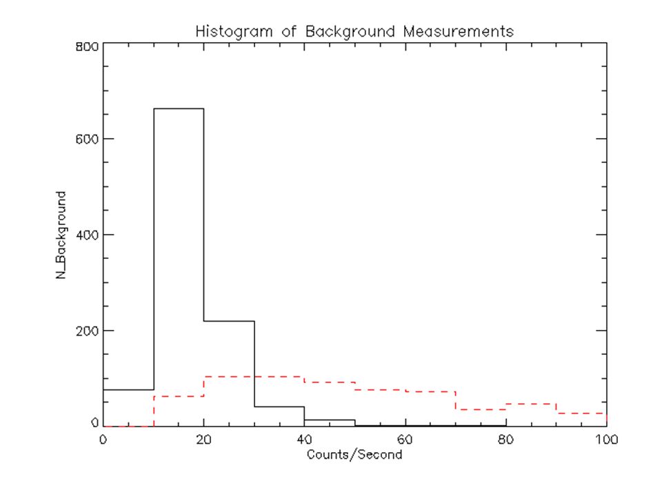
7. Figure 2: Is a histogram of the background rate from 3 to 6 keV used for the fits. The red dashed line is the histogram of the rate for the fits. The non-solar background is measured for 5 minute periods before and after the daylight portion of each orbit. Since the RHESSI background level is determined mostly by spacecraft position, we created a database of all of the pre and post daylight intervals for the mission. The background level used in each spectral fit was taken from the saved background interval with a spacecraft position closest to the position for the fit interval. For those intervals with no good position match, the pre or post daylight background closest in time was used. As long as the intervals in which the spacecraft is at high latitude are avoided, the background doesn’t vary much, as can be seen.

9. Figure 3: The top plot is the measured Emission Measure in units of 10^47 cm^(-3). The bottom plot is the Temperature in MK. The dashed red line is the daily sunspot number,normalized to a peak of 6, which is used here a a measure of solar activity. Thirty-four of the 1000 measurements returned 0 for EM and T; these had total count rates in the 3-12 keV band less than the background rate. The zero measurements are concentrated at times with low activity. Unfortunately it is difficult to get “quiet” sun measurements during times of high activity, so there are gaps in the measurements during active periods.

11. Figure 4: These are histograms of the EM and T measurements. The emission measures are concentrated at the low end; the temperatures are typically between 6 and 8 MK. ***Note on spectral fitting procedures: The spectral fits are obtained using software developed for ISEE-3/ICE, YOHKOH and ULYSSES. The abundances for the different ionic species are the default values used in the SSW program MEWE_SPEC, which are adapted from Meyer, J.-P., 1985 Apj. Suppl., 57, 173.

12. The Full-sun Differential Emission Measure from 1 to 10 MK Using SXI and RHESSI data. RHESSI only observes the hottest part of the solar DEM; in order to get a better handle on the DEM, we have done some preliminary work combining GOES 12-SXI data and RHESSI. SXI data and analysis tools can be found at the NOAA website: http://sec.noaa.gov/sxi/index.html. The SXI has multiple analysis filters with different broad-band temperature responses. SXI takes one image per minute, typically with the ‘P_MED’ and ‘B_THN’ filters. Once every 6 hours, the SXI cycles through all of its filters. We found 4 intervals from the 1000 used for this study that were close enough to a full set of SXI images for a try at a multi-instrument DEM calculation.

14. Figure 5: This shows normalized T response curves for two of the SXI filters and two RHESSI channels. The ‘P_MED’ SXI filter has a broad response with a peak at about 3.9 MK. The ‘B_MED’ filter has a broader response that peaks at 10 MK but has a noticeable response at much lower T. The RHESSI channels have response curves that increase rapidly with increasing T. If there is any high-T plasma present, it will have a dominant effect on the RHESSI count rate. For the DEM calculations, the full image is used; since we have not yet imaged the RHESSI sources, a spatially resolved DEM cannot be used. The DEM calculation is done using the histogram- DEM method described in McTiernan, Fisher & Li, 1999, Apj 514, 472 for YOHKOH SXT and BCS.

16. Figure 6: These are plots of the DEM for the four “quiet” intervals with good SXI coverage. Nothing wildly surprising, the DEM is high at low T and decreases with increased T. The results would be similar to a model of loops heated by nanoflares presented by Klimchuk and Cargill Apj 553, 440, except for the fact that the Klimchuk-Cargill DEM has a peak near 3 MK, and this DEM does not show a peak. It is possible that a DEM calculation concentrating on one active region, instead of the whole sun, could show such a peak. It is also true that these measurements were obtained at relatively quiet times and the temperature may just be that low.

17. In any case, verification of solar heating models will require DEM’s for individual active regions and the inclusion of lower T (e.g. TRACE) observations with the SXI and RHESSI data to extend the calculation. The first step will be to try to identify the positions of the “quiet sun” RHESSI sources.

18. Conclusions: There is typically a high T(6-8) MK source present on the sun even for periods with no observable flare activity. The high T emission is greater during active periods, and can disappear during quiet periods. We can obtain DEM measurements of the quiet sun using SXI and RHESSI, but more work is needed for these to be useful