1. 統計計算與模擬 政治大學統計系余清祥 2003 年 6 月 9 日 ~ 6 月 10 日 第十六週：估計密度函數 http://csyue.nccu.edu.tw

2. Density Estimation Estimate the density functions without the assumption that the p.d.f. has a particular form.  The idea of estimating c.d.f. (i.e., F(x 0 )) is to count the number of observations not larger than x 0. Since the p.d.f. is the derivative of c.d.f., the natural estimate of the p.d.f. would be However, this is likely not a good estimate since most points have zero density.

3. Therefore, we may want to assign a nonzero weight to points near points with observations. Intuitively, the weight should be larger if a point is close to a observation, but this is not necessary to be true.

4. Smoothing, a process of obtaining a corresponding smooth set of values from irregular set of observed values, is closely linked computationally to density estimation.

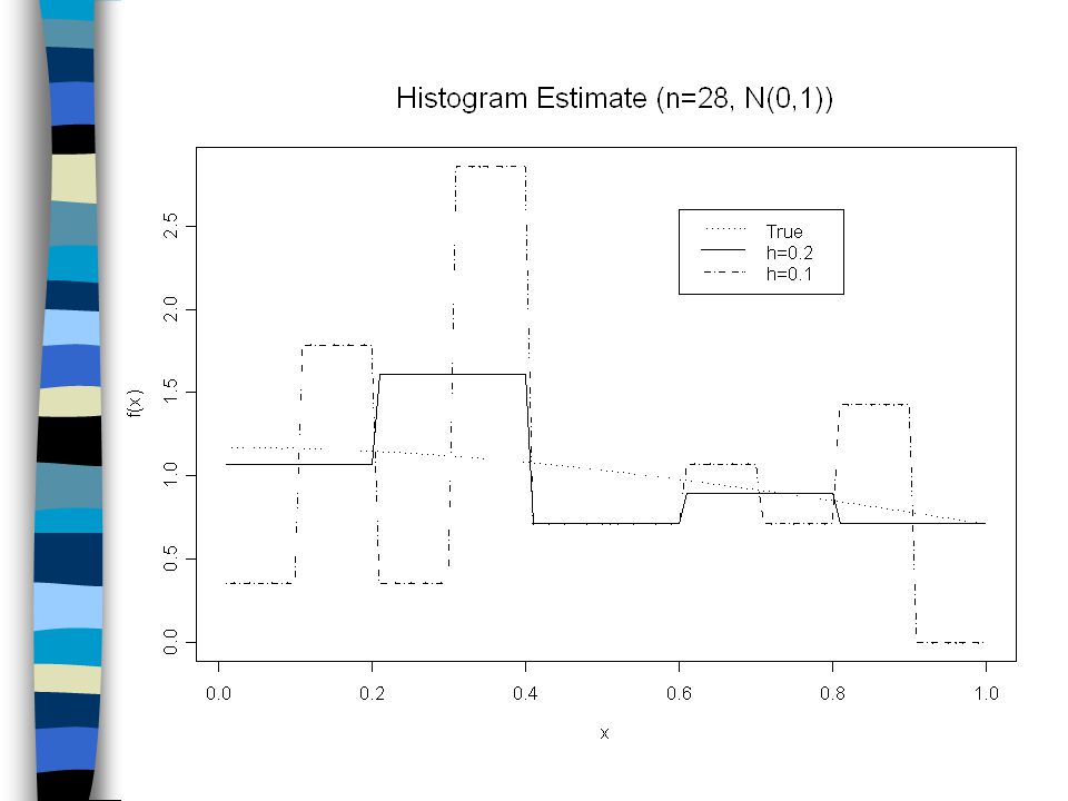
5. Histogram  The histogram is the simplest and most familiar method of a density estimator.  Break the interval [a,b] into m bins of equal width h, say Then the density estimate of is where n j is the number of observations in the interval

6. Notes: (1) The histogram density estimate looks like the sample c.d.f. and is a step function. (2) The smaller h is, the smoother the density estimate will be. However, given a finite number of observations, when h is smaller than most of the distances between two points, the density estimate would become more discrete. Q: What is the “optimal” choice of h? (The number of bins for drawing a histogram)

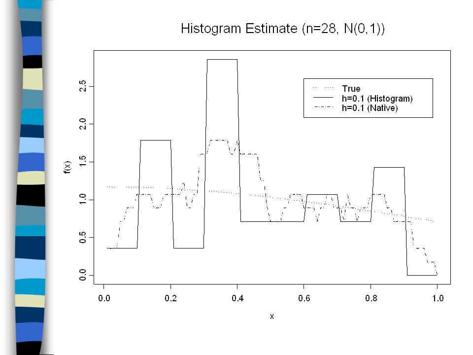
8. The Naïve Density Estimator  Instead of rectangle, allow the weight is centered on x. From Silverman (1986), where Because the estimate is constructed from a moving window of width 2h, it is also called a moving-window histogram.

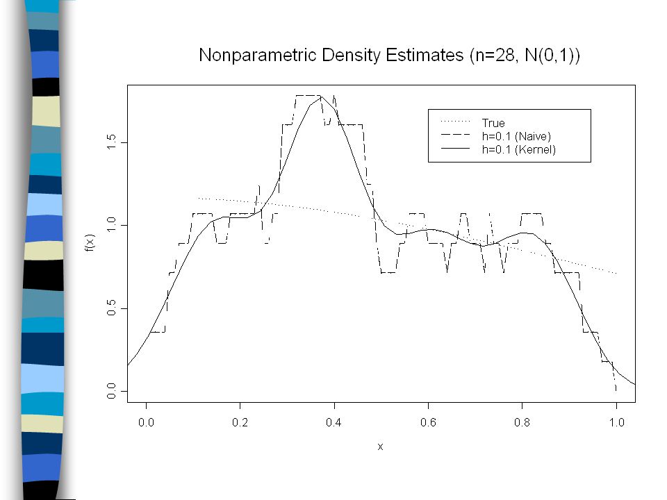
10. Kernel Estimator:  The naïve estimator is better than the histogram, since weight is based on distance between observations and x. However, it also has jumps (similar to the histogram estimate) at the observation points. By modifying the weight function w(  ) to be more continuous, the raggedness of the naïve estimate can be overcome.

11.  The kernel estimate is as following: where is the kernel of the estimator.  Usual choices of kernel functions: Guassian (i.e., normal), Cosine, Rectangular, Triangular, Lapalce. Note: The choice of the bandwidth (i.e., h) is more critical than the kernel function.

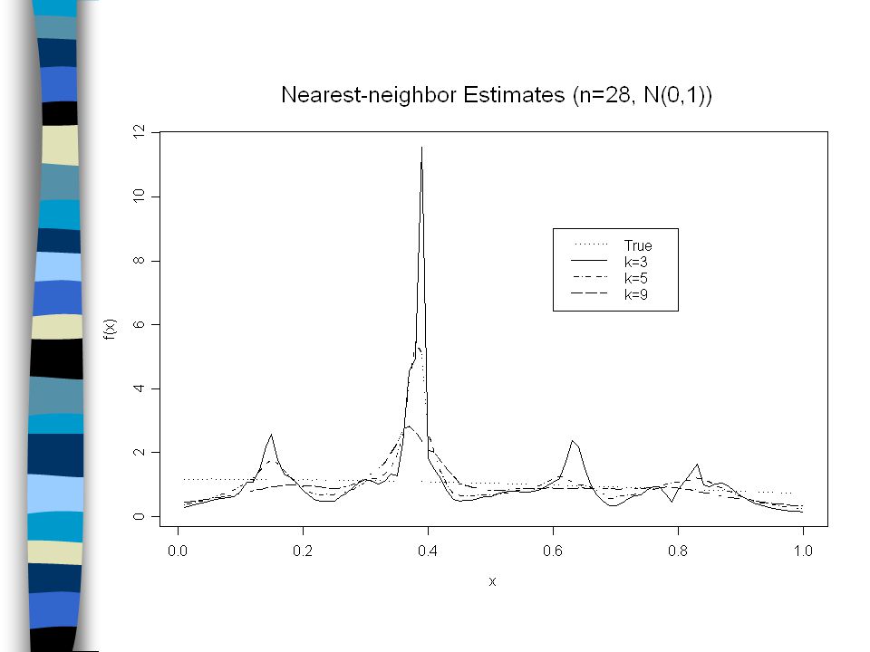
13. Nearest-neighbor Estimator: (NNE)  Another usage of observations is to use the concept of “nearness” between points and observations. But, instead of distance, the nearness is measured according to the number of other observations between a point and the specified observation. For example, if x 0 and x are adjacent in the ordering, then x is said to be 1-neighbor of x 0. If another observation between x 0 and x, then x is said to be 2-neighbor of x 0.

14.  The nearest-neighbor density estimates are based on averages of the k nearest neighbors in the sample to the point x: where is the half-width of the smallest interval centered at x containing k data points. Note: Unlike kernel estimates, the NNE use variable-width window.

16. Linear Smoother:  The goal is the smooth estimates of a regression function A well-known example is the ordinary linear regression, where the fitted values are  A Linear Smoother is the one which the smooth estimate satisfies the following form: where S is an n  n matrix depending on X.

17. Running Means:  The simplest case is the running-mean smoother which computes by averaging y j ’s for which x j falls in a neighborhood of x i.  One possible choice of the neighborhood N i is to adapt the idea in Nearest-neighbor where N i is the one with points x j for which |i – j|  k. Such a neighborhood contains k points to the left and k points to the right. (Note: The two tails have fewer points and could be less smooth.)

18. Note: The parameter k, called the span of the smoother, controls the degree of smoothing. Example 2. We will use the following data to demonstrate the linear smooth methods introduced in this handout. Suppose that where the noise  i is normally distributed with mean 0 and variance 0.04. Also, the setting of X is 15 points on [0,0.3], 10 points on [0.3,0.7] and 15 points on [0.7,1].

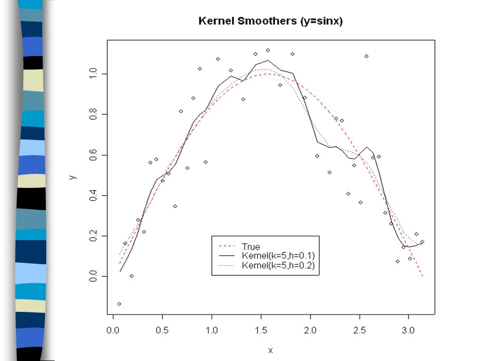
20. Kernel Smoothers  The product of a running-mean smoother is usually quite unsmooth, since observations are getting equal weight regardless their distance to the point to be estimated. The kernel smoother with kernel K and window 2h uses where

21. Notes: (1) If the kernel is smooth, then the resulting output will also be smooth. The kernel smoother estimate can thus be treated as a weighted sum of the (smooth) kernels, (2) The kernel smoothers also cannot correct the problem of bias in the corners, unless the weight of observations can be negative.

23. Spline Smoothing:  For the linear smoothers discussed previously, the smoothing matrix S is symmetric, has eigenvalues no greater than unity, and produce linear functions.  The smoothing spline is to select so as to minimize the following objective function: where  0 and M  C 3.

24. Note: Two terms of the right-hand side of the objective function usually represent constraints opposite to each other.  The first term measures how far the smoothers differ from the original observations.  The second term, also known as roughness penalty, measures the smoothness of the smoothers. Note: Methods which minimize the objective function are called penalized LS methods.

25. What are Splines?  Spline functions, often called splines, are smooth approximating functions that behave very much like polynomials.  Splines can be used for two purposes: (1) Approximate a given function (Interpolation) (2) Smooth values of a function observed with noise Note: We use terms “interpolating splines” and “smoothing splines” to distinguish.

26.  Loosely speaking, a spline is a piecewise polynomial function satisfying certain smoothness at the joint points. Consider a set of points, also named the set of knots, with  Piecewise-polynomial representations:

27. Q: Is it possible to use a polynomial to do the job?

28.  A cubic spline can be expressed as which can also be expressed as where

29. Example 2. (continued)  We shall use cubic splines with knots at {0,  /3,2  /3,  } and compare the results of smoothing for different methods. Note: There are also other smoothing methods available, such as LOWESS and running median (i.e., nonlinear smoothers), but we won’t cover these topics in this class.