1. Chapter 4 Roots of Equations
The values of x that satisfy the condition are termed the roots of the function; these roots are the solution to the equation f(x) = 0.
The general second-order polynomial:
Solutions (roots):

2. The roots for third-order polynomial can also be found analytically
The roots for third-order polynomial can also be found analytically. No general solution exists for other higher-order polynomials.
It is more difficult to obtain analytical roots of nonpolynomial, nonlinear fucntions. E.g.
cannot be solved analytically.

3. Roots of Some Selected Functions
(a) No Roots
(b) One Root

4. Two Roots
Three Roots

5. Eigenvalue Analysis
The eigenvalues or characteristic values, are the values, usually denoted as , for which the following matrix system has a nonzero (i.e., nontrivial) solution vector X :
The matrices A and I are of the order n n, with I being an identify diagonal matrix.
We have to solve the characteristic equation:
The roots  are the eigenvalues.

6. Example: Characteristic Equationor
Then, we have to solve the above equation.

7. Direct-Search Method It is a trial-and-error approach.
We do not get an exact value for the root; we obtain only an estimate of the root (to within some specified degree of precision).
Step 1: Specify a range or interval for x within the root is assumed to occur. Smaller initial intervals will require fewer calculations to obtain the root to the desired accuracy.
Step 2: Divide the interval into smaller, uniformly spaced subintervals. The size of these subintervals will be dictated by the required precision for the estimate of the root.

8. Step 3: Search through all subintervals until the subinterval containing the root is located.
If a root does not lie within the subinterval [A,B], then f(A) and f(B) have the same sign.
(a) no roots in the interval [A, B]

9. (b) no roots in the interval [A, B]
(c) one root in the interval [A, B]
(d) one root in the interval [A, B]

10. The direct-search method will find the roots of any function as long as all the roots are real and within the specified interval.
Some roots might be missed entirely if the subinterval is so large that more than one root occurs in a single subinterval.
The direct-search method assumes that there is one and only one root within each subinterval.
If there is an even number of roots within the search interval, then f(A) and f(B) will have the same sign, and the search process will miss the roots within the interval.

11. Multiple roots
The multiple roots cannot be determined by the direct-search method.
Multiple Roots

12. Point of Discontinuity
The direct-search method cannot find the root of a function that has a discontinuity at a point within [A,B].
Point of Discontinuity

13. Example: Finding Eigenvalues
f()
0.0
-0.504
0.1
-0.302
0.2
-0.153
0.3
-0.053
0.4
0.006
0.5
0.199
0.6
0.021
0.7
-0.011
0.8
-0.061
0.9
-0.122
1.0
-0.190
1.1
-0.257
1.2
-0.319
1.3
-0.368
1.4
-0.400
1.5
-0.407
1.6
-0.385
1.7
-0.326
1.8
-0.226
1.9
-0.077
2.0
0.125
Roots:
We can get better estimate with linear interpolation.

14. Bisection Method
Step 1: For the interval of x from the starting point xs to the end point xe, locate the midpoint xm at the center of the interval.

15. Step 2: Evaluate the values of f(xs), f(xm), and f(xe).
Step 3: Compute f(xs)f(xm) and f(xm)f().
If f(xs)f(xm) <0, then xs < root < xm.
If f(xm)f(xe) <0, then xm < root <xe.
Step 4: . Check for convergence. If the convergence criterion (that is, tolerance) is satisfied, then use xm as the final estimate of the root. Otherwise, go to Step 1.
The bisection method will always converge on the root, provided that only one root lie within the starting interval for x.

16.  Error Analysis and Convergence Criterion
 The absolute value of the difference (d)
 The relative percent error (r)
 The true error (t) in the ith iteration

17. Example: Bisection Method
We are interested in finding the roots within the interval 3.75  x  5.00 to a relative accuracy as an absolute value between successive iterations of 0.01.
The absolute value of the error is given in the last column of Table 4-2.
The final estimate of the root is

18. Table 4-2 Example Polynomial Solved Using the Bisection Method
Iteration i xs xm xe
f(xs)
f(xm)
f(xe)
Subinterval Containing Root
Error d
f(xs) f(xm)
f(xm) f(xe) 1
3.750
4.375
5.000
-6.830
12.850
42.000 - + — 2
4.062
1.903
0.313 3
3.906
-2.724
0.156 4
3.984
-0.477
0.078 5
4.023
0.696
0.039 6
4.004
0.120
0.019 7
3.994
-0.180
0.010
The true root=4
The true accuracy of the estimated root is or, in relative terms, 0.15%.

19. Newton-Raphson Iteration
The Newton-Raphson iteration method is a faster method for converging on a single root of a function.
It uses the linear portion of a Taylor series:

20. General formula of Newton-Raphson method:

21. Newton-Raphson Method

22. Example: Newton-Raphson Method
The derivative:
Assume an initial estimate of the root x0=6.0.

23. Error Analysis (xt: true root)
Iteration i xi
xi - xi-1
xi – xt
6.0000 ─
2.0000 1
4.6977
1.3023
0.6977 2
4.1289
0.5688
0.1289 3
4.0057
0.1232
0.0057 4
4.0000
0.0000
For this case, the convergence criterion xi - xi-1 yeilds a conservative estimate of the true error.
The solution should be checked by substituting the calculated root into the function.

24. Nonconvergence of Newton-Raphson Method
Newton-Raphson method usually converges to a root faster than does the bisection method.
Newton-Raphson method may fail to converge.
In a computer program, an iteration counter should be used to terminate the root searching procedure when some preseclected number of iteration has been exceeded.

25. Nonconvergence Cases
Case 1: If the initial estimate is selected such that the derivative of the function equals zero.
An example case of f ’(xi) = 0 :

26. Case 2:

27. Case 3: A large number of iterations will be required if f’(xi) is much larger than f(xi). In such cases, 　　 is small, which leads to a small adjustment at each iteration.

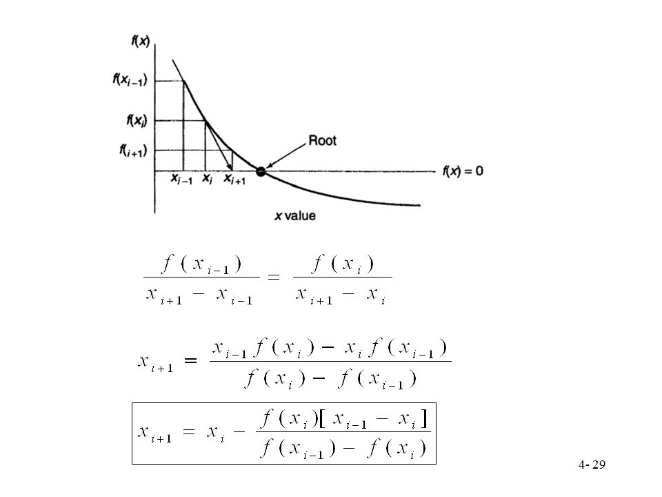
28. Secant Method
The secant method is similar to the Newton-Raphson method, with the difference that the derivative f’(x) is numerically evaluated, rather than computed analytically.
The secant method requires two initial estimates of a root.

30.  Example: Secant Method
Two initial estimates of x0 = 0 and x0 = 1.
The method converges to a root of

31. Secant Method Iteration i f(xi-1) xi Comments 1 Initial condition1
Initial condition 2 3 4 5
2.81E-06 6
4.11E-10 7
- 2.20E-16 8 9

32. Polynomial Reduction
If the polynomial f(x)=0 and root x1 is a root of f(x), then there is a reduced polynomial f*(x) such that (x-x1)f*(x) = 0, where f*(x) = f(x)/(x-x1).
After a root of a polynomial is found, we can find the next root by calculating the root of the reduced polynomial.

33. Example: Polynomial Reduction
Suppose, with the Newton-Raphson method, one root of the polynomial of was found to be x1 = 4. This polynomial can be reduced as
can be used to find additional roots.
The error in x1 will lead to error in the coefficients of the reduced equation and thus, all roots found subsequently.

34. Example : Eigenvalue Problem
Suppose the first root =1.942 is found. The reduced polynomial will have a little error.

35. Synthetic Division nth-order polynomial:
dividing it by an initial estimate of the root x0:
where R0 is the remainder.
The reduced polynomial hn-1(x) is given by:

36. hn-1(x) is also reduced:
where R1 is the remainder. gn-2(x) can be written as
We get
We have fn(x0) = R0 and f’n(x0) = R1.

37. Based on the Newton-Raphson method, we get
General formula of the synthetic division method:
Newton-Raphson method and the synthetic division method give the same answer.
New-Raphson method requires the first derivative of the polynomial. The synthetic division method requires two polynomial reductions.

38. Programming Considerations
It can be shown:

39. Similarly,
The remainders R0 and R1:

40. Synthetic Division Procedure
Step 1: Input n, x0, bj for j = 0, 1, … , n.
Step 2:
Step 3:
Step 4:

41. Step 5: Step 6: Check for convergence :
a. if │xi+1 - xi│ tolerance, discontinue the 　　　iteration and use xi+1 as the best estimate 　　　of the root; or
b. if │xi+1 - xi│ tolerance, set xi = xi+1 and 　　　return to Step 2 and continue the iteration 　　　process.

42. Example: Synthetic Division
An initial estimate x0=6, the first reduction:

43. The second reduction:
Thus the revised estimate is
After six iterations, the root to seven significant digits is 4.

44. Table 4-6 Synthetic Division
Parameter
Iteration 0
Iteration 1
Iteration 2
Iteration 3
Iteration 4
Iteration 5 xi 6 4 R0
112
1.54E-09 R1 86 30 b3 1 b2 -1 b1
-10 b0 -8 C2 c1 5 3 c0 20 2 d1 d0 11 7

45. Multiple Roots
Multiple roots at x=1, and one root at x=5

46. Even multiple roots result in a tangent f(x) to the x axis, whereas odd multiple roots result in a function f(x) that crosses the x axis with an inflection point at the root, that is, a point where the function changes curvature.
The bisection method has difficulties with multiple roots because the function does not change sign at even multiple roots.
The Newton-Raphson and secant method have difficulties because f’(x)=0 at a multiple root.
Since f(x) reaches zero faster than f’(x) as x approaching the multiple root, we can check the condition f(x)=0 and terminate the computations before reaching f’(x)=0.

47. Systems of Nonlinear Equations
Form of the two-variable system:
fi(x,y) = 0
where the subscript i denotes the equation number, and both x and y are independent variables.
The number of equations should be equal to the number of variables.
A two-variable system of nonlinear equations:

48. Jacobi Method
Using initial estimates, the transformed equations are solve iteratively until the solution converges.
Using initial estimates x = y = 3:

49. Using x = and y = 3:
For the second iteration, x = and y = :
Using x = and y = :
Finally, the solution would converge:
x = y = 1.82.

50. Table: Nonlinear System Results
Iteration i x y 1 2 3 4 5 6 7 8 9 10
Iteration i x y 11 12 13 14 15 16 17 18 19 20

51. Figure: Nonlinear system results