11 PERFECT COMPETITION CHAPTER.

11 PERFECT COMPETITION CHAPTER

Objectives After studying this chapter, you will able to
Define perfect competition Explain how price and output are determined in perfect competition Explain why firms sometimes shut down temporarily and lay off workers Explain why firms enter and leave the industry Predict the effects of a change in demand and of a technological advance Explain why perfect competition is efficient Students find this topic challenging. Part of their problem is that it builds on the cost curves of the previous chapter and many of them still have only a shaky grasp of that material. So emphasize the cumulative nature of economics and remind the students of the huge payoff from mastering material a bite at a time. You can help your students by emphasizing the two primary goals of this chapter: (1) To derive the market supply curve in a competitive industry and (2) to deepen your students’ understanding of how competition among self-interested consumers and producers moves resources from where they are less valued to where they are more valued and to an efficient allocation. Explain that although Chapter 3 (Demand and Supply) and Chapter 5 (Efficiency and Equity) covered these same topics, they did so at a level that is one step removed from the decision makers. Remind the students that they’ve seen how consumer decisions lead to the best use of a household’s income. Point out that they are now going see how producer decisions are made and how they interact with consumer decisions. You might like to use the metaphor that the chapter strips away more of the veil that hides the invisible hand.

Competition Perfect competition is an industry in which:
Many firms sell identical products to many buyers. There are no restrictions to entry into the industry. Established firms have no advantages over new ones. Sellers and buyers are well informed about prices. The range of market types. Remind the students of what they learned in Chapter 9 about the spectrum of markets that range from perfect competition to monopoly. The perfect competition model serves as a benchmark and its predictions work in a wide range of real markets. Set the scene for appreciating the power of the perfect competition model with a physical analogy. Explain that physicists often use the model of a “perfect vacuum” to understand our physical world. For example, to predict how long it will take a 50 pound steel ball to hit the ground if it is dropped from the top of the Empire State Building, you will be very close to the actual time if you assume a perfect vacuum and use the formula that applies in that case. Friction from the atmosphere is obviously not zero, but assuming it to be zero is not very misleading. In contrast, if you want to predict how long it will take a feather to make the same trip, you need a fancier model! Economists use the model of “perfect competition” in a similar way to understand our economic world. Emphasize to students that although no real world industry meets the full definition of perfect competition, the behavior of firms in many real world industries and the resulting dynamics of their market prices and quantities can be predicted to a high degree of accuracy by using the model of perfect competition.

Competition How Perfect Competition Arises Perfect competition arises:
When firm’s minimum efficient scale is small relative to market demand so there is room for many firms in the industry. And when each firm is perceived to produce a good or service that has no unique characteristics, so consumers don’t care which firm they buy from.

Competition Price Takers
In perfect competition, each firm is a price taker. A price taker is a firm that cannot influence the price of a good or service. No single firm can influence the price—it must “take” the equilibrium market price. Each firm’s output is a perfect substitute for the output of the other firms, so the demand for each firm’s output is perfectly elastic. Price taking. Be sure to spend a few minutes providing intuition to ensure that your students understand why firms in perfect competition are price takers: They can offer to sell for a lower price, but they’re giving profits away; and they can ask for a higher price, but no one will pay. You might like to note that if the market is not in equilibrium, the firm isn’t a price taker. If there is a shortage, firms can get away with a higher price and they ask for more. That’s how prices rise. If there is a surplus, firms offer a lower price to move their product. That’s how prices fall. But in equilibrium, there is nothing to do but take the going price. And competitive markets get to equilibrium fast.

Competition Economic Profit and Revenue
The goal of each firm is to maximize economic profit, which equals total revenue minus total cost. Total cost is the opportunity cost of production, which includes normal profit. A firm’s total revenue equals price, P, multiplied by quantity sold, Q, or P  Q.

Competition A firm’s marginal revenue is the change in total revenue that results from a one-unit increase in the quantity sold. Figure 11.1 illustrates a firm’s revenue curves.

Competition Figure 11.1(a) shows that market demand and supply determine the price that the firm must take.

Competition Figure 11.1(b) shows the demand curve for the firm’s product, which is also its marginal revenue curve.

Competition Because in perfect competition the price remains the same as the quantity sold changes, marginal revenue equals price.

Competition Figure 11.1(c) shows the firm’s total revenue curve.

The Firm’s Decisions in Perfect Competition
A perfectly competitive firm faces two constraints: A market constraint summarized by the market price and the firm’s revenue curves A technology constraint summarized by firm’s product curves and cost curves (like those in Chapter 10).

The perfectly competitive firm makes two decisions in the short run: Whether to produce or to shut down. If the decision is to produce, what quantity to produce. A firm’s long-run decisions are: Whether to increase or decrease its plant size. Whether to stay in the industry or leave it.

Profit-Maximizing Output A perfectly competitive firm chooses the output that maximizes its economic profit. One way to find the profit maximizing output is to look at the firm’s the total revenue and total cost curves. Figure 11.2 on the next slide looks at these curves along with the firm’s total profit curve. Do firms really choose the output that maximizes profit? It is useful to explain to your students that many big firms routinely make tables using spreadsheets of total revenue, total cost, and economic profit—and make graphs—similar to those in Figure But most firms, and certainly most small firms like Cindy’s sweater knitting firm, don’t make such calculations. Nonetheless, they do make their decisions at the margin. They can figure out how much it will cost to hire one more worker and how much output that worker will produce. So they can figure out their marginal cost—wage rate divided by marginal product. They can compare that number with the price. They are choosing at the margin.

Part (a) shows the total revenue, TR, curve. Part (a) also shows the total cost curve, TC, which is like the one in Chapter 10. Total revenue minus total cost is profit (or loss), shown in part (b).

Profit is maximized when the firm produces 9 sweaters a day. At low output levels, the firm incurs an economic loss—it can’t cover its fixed costs.

At intermediate output levels, the firm earns an economic profit. At high output levels, the firm again incurs an economic loss—now it faces steeply rising costs because of diminishing returns.

Marginal Analysis The firm can use marginal analysis to determine the profit-maximizing output. Because marginal revenue is constant and marginal cost eventually increases as output increases, profit is maximized by producing the output at which marginal revenue, MR, equals marginal cost, MC. Figure 11.3 on the next slide shows the marginal analysis that determines the profit-maximizing output.

If MR > MC, economic profit increases if output increases. If MR < MC, economic profit decreases if output increases. If MR = MC, economic profit decreases if output changes in either direction, so economic profit is maximized.

Profits and Losses in the Short Run Maximum profit is not always a positive economic profit. To determine whether a firm is earning an economic profit or incurring an economic loss, we compare the firm’s average total cost, ATC, at the profit maximizing output with the market price. Figure 11.4 on the next slide shows the three possible profit outcomes.

In part (a) price equals ATC and the firm earns zero economic profit (normal profit). Operating a business at zero economic profit. Students are often skeptical that a zero economic profit is an acceptable outcome for an entrepreneur. The key is to reinforce the meaning of normal profit. A rational decision is one that is based on a weighing of the full opportunity cost of each alternative against its full benefits—for a firm weighing the total revenue against the opportunity cost for each alternative. Opportunity cost includes the benefits from forgone opportunities as well as explicit costs. One of these forgone opportunities is that of the entrepreneur pursuing her/his next best activity. The value of this forgone opportunity is normal profit. So, when a firm earns zero economic profit, the entrepreneur earns normal profit and enjoys the same benefits as those available in the next best activity. There is no incentive to change to the next best activity.

In part (b), price exceeds ATC and the firm earns a positive economic profit.

In part (c) price is less than ATC and the firm incurs an economic loss—economic profit is negative and the firm does not even earn normal profit. Operating a business at a loss. Students often have a hard time understanding why operating at an economic loss can be the best action. The key is appreciating that: The firm’s short-run decisions are made after some irrevocable commitments have generated sunk costs. The firm considers only avoidable costs when making decisions. Unavoidable costs have no impact on the decision. So for the firm to produce its revenues need only exceed avoidable costs, not total costs. The profit maximization goal doesn’t require the firm to earn a positive economic profit in the short run.

The Firm’s Short-Run Supply Curve A perfectly competitive firm’s short run supply curve shows how the firm’s profit-maximizing output varies as the market price varies, other things remaining the same. Because the firm produces the output at which marginal cost equals marginal revenue, and because marginal revenue equals price, the firm’s supply curve is linked to its marginal cost curve. But there is a price below which the firm produces nothing and shuts down temporarily.

Temporary Plant Shutdown If price is less than the minimum average variable cost, the firm shuts down temporarily and incurs a loss equal to total fixed cost. This loss is the largest that the firm must bear. If the firm were to produce just 1 unit of output at price below average variable cost, it would incur an additional (and avoidable) loss. Temporary shutdown. In our experience, this topic is the hardest for the students to understand. You can help them with the intuition by pointing out that the rationale for temporary shutdown isn’t confined to perfect competition and that they can see the phenomenon right around the corner. Many restaurants close on Sunday evening and Monday. Many hairdressers close on Sunday and Monday. Why? Your students will easily figure out that total revenue is less than total variable cost and equivalently that price is less than average variable cost. The mechanics of the shutdown analysis will be a lot easier to explain once the students have thought about these real situations with which they are familiar.

The shutdown point is the output and price at which the firm just covers its total variable cost. This point is where average variable cost is at its minimum. It is also the point at which the marginal cost curve crosses the average variable cost curve. At the shutdown point, the firm is indifferent between producing and shutting down temporarily. It incurs a loss equal to total fixed cost from either action.

If the price exceeds minimum average variable cost, the firm produces the quantity at which marginal cost equals price. Price exceeds average variable cost, and the firm covers all its variable cost and at least part of its fixed cost. When to increase and when to decrease output. Students need repeated reminders that to determine whether a firm can increase profit by changing output, price, and marginal cost are the only things to consider. Questions that throw average total cost into the mix often cause confusion.

Figure 11.5 shows how the firm’s short-run supply curve is constructed. If price equals minimum average variable cost, $17 in this example, the firm is indifferent between producing nothing and producing at the shutdown point, T.

If the price is $25, the firm produces 9 sweaters a day, the quantity at which P = MC. If the price is $31, the firm produces 10 sweaters a day, the quantity at which P = MC. The blue curve in part (b) traces the firm’s short-run supply curve.

Short-Run Industry Supply Curve The short-run industry supply curve shows the quantity supplied by the industry at each price when the plant size of each firm and the number of firms remain constant.

The quantity supplied by the industry at any given price is the sum of the quantities supplied by all the firms in the industry at that price.

At a price equal to minimum average variable cost—the shutdown price—the industry supply curve is perfectly elastic because some firms will produce the shutdown quantity and others will produces zero.

Output, Price, and Profit in Perfect Competition
Short-Run Equilibrium Short-run industry supply and industry demand determine the market price and output. Figure 11.7 shows a short-run equilibrium at the intersection of the demand and supply curves.

A Change in Demand An increase in demand bring a rightward shift of the industry demand curve: the price rises and the quantity increases. A decrease in demand bring a leftward shift of the industry demand curve: the price falls and the quantity decreases.

Long-Run Adjustments In short-run equilibrium, a firm may earn an economic profit, earn normal profit, or incur an economic loss and which of these states exists determines the further decisions the firm makes in the long run. In the long run, the firm may: Enter or exit an industry Change its plant size

Entry and Exit New firms enter an industry in which existing firms earn an economic profit. Firms exit an industry in which they incur an economic loss. Figure 11.8 on the next slide shows the effects of entry and exit.

As new firms enter an industry, industry supply increases. The industry supply curve shifts rightward. The price falls, the quantity increases, and the economic profit of each firm decreases.

As firms exit an industry, industry supply decreases. The industry supply curve shifts leftward. The price rises, the quantity decreases, and the economic profit of each firm increases.

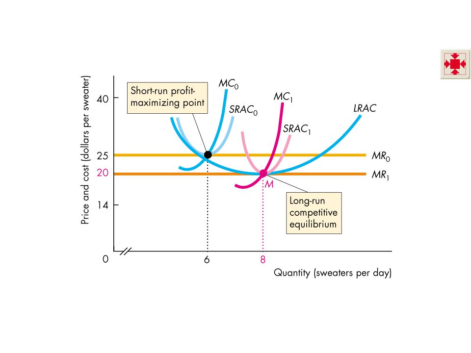
Changes in Plant Size Firms change their plant size whenever doing so is profitable. If average total cost exceeds the minimum long-run average cost, firms change their plant size to lower costs and increase profits. Figure 11.9 on the next slide shows the effects of changes in plant size.

If the price is $25, firms earn zero economic profit with the current plant.

But if the LRAC curve is sloping downward at the current output, the firm can increase profit by expanding the plant.

As the plant size increases, short-run supply increases, the price falls, and economic profit decreases.

Long-run equilibrium occurs when the firm is producing at the minimum long-run average cost and earning zero economic profit.

Long-Run Equilibrium Long-run equilibrium occurs in a competitive industry when: Economic profit is zero, so firms neither enter nor exit the industry. Long-run average cost is at its minimum, so firms don’t change their plant size.

Changing Tastes and Advancing Technology
A Permanent Change in Demand A decrease in demand shifts the demand curve leftward. The price falls and the quantity decreases. Watching the work of the invisible hand. The power of the market to make firms respond to consumers’ changing demands become visible to the student in this section. When you teach this material, do the analysis with a specific (and current/recent) example with which the students can identify. Computers and ISPs are good for an increase in demand. Audio tapes are good for a decrease in demand.

Starting from a position of long-run equilibrium, the fall in price puts the price below each firm’s minimum average total cost and firms incur an economic loss.

Economic losses induce exit, which decreases short-run supply and shifts the short-run industry supply curve leftward.

As industry supply decreases, the price rises and the market quantity continues to decrease.

With a rising price, each firm that remains in the industry increases production in a movement along the firm’s marginal cost curve (short-run supply curve).

A new long-run equilibrium occurs when the price has risen to equal minimum average total cost so that firms do not incur economic losses, and firms no longer leave the industry.

The main difference between the initial and new long-run equilibrium is the number of firms in the industry.

In the new equilibrium, a smaller number of firms produce the equilibrium quantity.

A permanent increase in demand has the opposite effects to those just described and shown in Figure 11.9. An increase in demand shifts the demand curve rightward. The price rises and the quantity increases. Economic profit induces entry, which increases short-run supply and shifts the short-run industry supply curve rightward. As industry supply increases, the price falls and the market quantity continues to increase.

With a falling price, each firm decreases production in a movement along the firm’s marginal cost curve (short-run supply curve). A new long-run equilibrium occurs when the price has fallen to equal minimum average total cost so that firms do not earn economic profits, and firms no longer enter the industry. The main difference between the initial and new long-run equilibrium is the number of firms in the industry. In the new equilibrium, a larger number of firms produce the equilibrium quantity.

External Economics and Diseconomies The change in the long-run equilibrium price following a permanent change in demand depends on external economies and external diseconomies. External economies are factors beyond the control of an individual firm that lower the firm’s costs as the industry output increases. External diseconomies are factors beyond the control of a firm that raise the firm’s costs as industry output increases.

In the absence of external economies or external diseconomies, a firm’s costs remain constant as industry output changes. Figure illustrates the three possible cases and shows the long-run industry supply curve, which shows how the quantity supplied by an industry varies as the market price varies after all the possible adjustments have been made, including changes in plant size and the number of firms in the industry.

Figure 11.11(a) shows that in the absence of external economies or external diseconomies, the price remains constant when demand increases.

Figure 11.11(b) shows that when external diseconomies are present, the price rises when demand increases.

Figure 11.11(c) shows that when external economies are present, the price falls when demand increases.

Technological Change New technologies are constantly discovered that lower costs. A new technology enables firms to producer at a lower average cost and lower marginal cost—firms’ cost curves shift downward. Firms that adopt the new technology earn an economic profit.

New-technology firms enter and old-technology firms either exit or adopt the new technology. Industry supply increases and the industry supply curve shifts rightward. The price falls and the quantity increases. Eventually, a new long-run equilibrium emerges in which all the firms use the new technology, the price has fallen to the minimum average total cost, and each firm earns normal profit.

The adjustment process as old-technology firms exit or adopt the new technology and new-technology firms enter can create great changes in local geographic prosperity. Some regions experience economic decline while others experience economic growth.

Competition and Efficiency
Efficient Use of Resources Resources are used efficiently when no one can be made better off without making someone else worse off. This situation arises when marginal benefit equals marginal cost. Pulling it all together In this section, you can show your students what they’ve learned and pull together the entire course to date. Begin by reiterating the two primary goals of this chapter and then note that you are now dealing with the second goal. Emphasize that the pressures of competition force self-interested firms to produce incredible long run results: Each firm produces at the lowest possible average total cost –at the minimum point of the long run average cost curve, Consumers pay the lowest possible price that keeps firms in business—P = minimum ATC. Each firm uses the least-cost technology, Firms produce the efficient quantity—price, which equals marginal benefit equals marginal cost. The forces of competition, which Adam Smith called an invisible hand, guide firms to produce output and charge prices that maximize the value of our scarce resources.

Choices, Equilibrium, and Efficiency We can describe an efficient use of resources in terms of the choices of consumers and firms coordinated in market equilibrium. We derive a consumer’s demand curve by finding how the best (most valued by the consumer) budget allocation changes as the price of a good changes. So consumers get the most value out of their resources at all points along their demand curves, which are also their marginal benefit curves.

We derive a competitive firm’s supply curve by finding how the profit-maximizing quantity changes as the price of a good changes. So firms get the most value out of their resources at all points along their supply curves, which are also their marginal cost curves. In competitive equilibrium, the quantity demanded equals the quantity supplied, so marginal benefit equals marginal cost. All gains from trade have been realized.

Competitive equilibrium is efficient only if there are no external benefits or costs. External benefits are benefits that accrue to people other than the buyer of a good. External costs are costs that are borne not by the producer of a good or service but by someone else.

Figure illustrates an efficient allocation of resources in a perfectly competitive industry. In part (a), each firm is producing at the lowest possible long run average total cost at the price P* and the quantity q*.

Figure 11.12(b) shows the market. Along the demand curve D = MB the consumer is efficient. Along the supply curve S = MC the producer is efficient.

The quantity Q* and price P* are the competitive equilibrium values. So competitive equilibrium is efficient. The consumer gains the consumer surplus, and the producer gains the producer surplus.

THE END

11 PERFECT COMPETITION CHAPTER.

Similar presentations

Presentation on theme: "11 PERFECT COMPETITION CHAPTER."— Presentation transcript:

Similar presentations

About project

Feedback

Log in

Auth with social network:

11 PERFECT COMPETITION CHAPTER.

Similar presentations

Presentation on theme: "11 PERFECT COMPETITION CHAPTER."— Presentation transcript:

Similar presentations

About project

Feedback