Download presentation
Presentation is loading. Please wait.

1
Relic Density at the LHC B. Dutta In Collaboration With: R. Arnowitt, A. Gurrola, T. Kamon, A. Krislock, D.Toback Phys.Lett.B639:46,2006, hep-ph/0608193 (Phys. Lett.B), To appear
, To appear.")
2
The signal to look for: 4 jet + missing E T SUSY in Early Stage at the LHC

3
Kinematical Cuts and Event Selection E T j1 > 100 GeV, E T j2,3,4 > 50 GeV M eff > 400 GeV (M eff E T j1 +E T j2 +E T j3 +E T j4 + E T miss ) E T miss > Max [100, 0.2 M eff ] Phys. Rev. D 55 (1997) 5520 Example Analysis
![Kinematical Cuts and Event Selection E T j1 > 100 GeV, E T j2,3,4 > 50 GeV M eff > 400 GeV (M eff E T j1 +E T j2 +E T j3 +E T j4 + E T miss ) E T miss > Max [100, 0.2 M eff ] Phys.](http://images.slideplayer.com/15/4794104/slides/slide_3.jpg "Rev. D 55 (1997) 5520 Example Analysis.")
4
SUSY scale is measured with an accuracy of 10-20% This measurement does not tell us whether the model can generate the right amount of dark matter. The dark matter content is measured to be 23% with an accuracy of less than 5% at WMAP Question: To what accuracy can we calculate the relic density based on the measurements at the LHC? Relic Density and M eff

5
We establish the dark matter allowed regions from the detailed features of the signals. We accurately measure the masses. We calculate the relic density and compare with WMAP. Strategy

6
Dark Matter Allowed Regions Neutralino-stau coannihilation region A-annihilation funnel region – This appears for large values of m 1/2 Focus point region – the lightest neutralino has a larger higgsino component We choose mSUGRA model. However, the results can be generalized.

7
+… In the stau neutralino coannihilation region Griest, Seckel ’91 Relic Density Calculation

8
In mSUGRA model the lightest stau seems to be naturally close to the lightest neutralino mass especially for large tan For example, the lightest selectron mass is related to the lightest neutralino mass in terms of GUT scale parameters: For larger m 1/2 the degeneracy is maintained by increasing m 0 and we get a corridor in the m 0 - m 1/2 plane. The coannihilation channel occurs in most SUGRA models with non-universal soft breaking, Thus for m 0 = 0, becomes degenerate with at m 1/2 = 370 GeV, i.e. the coannihilation region begins at m 1/2 = (370-400) GeV Coannihilation, GUT Scale
 GeV Coannihilation, GUT Scale.")
9
tan = 40, > 0, A 0 = 0 Can we measure M at colliders? Coannihilation Region

10
SUSY at LHC In Coannihilation Region of SUSY Parameter Space: Soft pppp Hard Final state: 3/4 s+jets +missing energy Signals

11
2. Use Counting Method (NOS-LS) & Ditau Invariant Mass (M ) to measure mass difference Use Hadronically Decaying and construct 3 observables 1.Sort τ’s by E T (E T 1 > E T 2 > …) and use OS-LS method to extract pairs from the decays 3. Measure the P T of the low energy Observables
 & Ditau Invariant Mass (M ) to measure mass difference Use Hadronically Decaying and construct 3 observables 1.Sort τ’s by E T (E T 1 > E T 2 > …) and use OS-LS method to extract pairs from the decays 3. Measure the P T of the low energy Observables.")
12
Since we are using 3 variables, we can measure M, Mgluino and the universality relation of the gaugino masses i.e. M gluino measured from the M eff method may not be accurate for this parameter space since the tau jets may pass as jets in the M eff observable. The accuracy of measuring these parameters are important for calculating relic density. SUSY Parameters

13
Version 7.69 (m 1/2 = 347.88, m 0 = 201.06) M gluino = 831 Chose di- pairs from neutralino decays with (a) | | < 2.5 (b) = hadronically-decaying tau Number of Counts / 1 GeV E T vis(true) > 20, 20 GeV E T vis(true) > 40, 20 GeV E T vis(true) > 40, 40 GeV E T > 20 GeV is essential! M vis in ISAJET

14
EVENTS WITH CORRECT FINAL STATE : 1 + 3j + E T miss APPLY CUTS TO REDUCE SM BACKGROUND (W+jets, …) E T miss > 100 GeV, E T j1 > 100 GeV, E T miss + E T j1 > 400 GeV ORDER TAUS BY P T & APPLY CUTS ON TAUS: WE EXPECT A SOFT AND A HARD P T > 40, 40, 20 GeV, LOOK AT PAIRS AND CATEGORIZE THEM AS OPPOSITE SIGN (OS) OR LIKE SIGN (LS) OS: FILL LOW OS P T HISTOGRAM WITH P T OF SOFTER FILL HIGH OS P T HISTOGRAM WITH P T OF HARDER LS: FILL LOW LS P T HISTOGRAM WITH P T OF SOFTER FILL HIGH LS P T HISTOGRAM WITH P T OF HARDER LOW OS HIGH OS LOW LS HIGH LS LOW OS-LS HIGH OS-LS Extracting Pairs from Decays E T miss + 1j + 3 Analysis Path
 E T miss > 100 GeV, E T j1 > 100 GeV, E T miss + E T j1 > 400 GeV ORDER TAUS BY P T & APPLY CUTS ON TAUS: WE EXPECT A SOFT AND A HARD P T > 40, 40, 20 GeV, LOOK AT PAIRS AND CATEGORIZE THEM AS OPPOSITE SIGN (OS) OR LIKE SIGN (LS) OS: FILL LOW OS P T HISTOGRAM WITH P T OF SOFTER FILL HIGH OS P T HISTOGRAM WITH P T OF HARDER LS: FILL LOW LS P T HISTOGRAM WITH P T OF SOFTER FILL HIGH LS P T HISTOGRAM WITH P T OF HARDER LOW OS HIGH OS LOW LS HIGH LS LOW OS-LS HIGH OS-LS Extracting Pairs from Decays E T miss + 1j + 3 Analysis Path")
15
E T miss + 1j + 3 Analysis Much smaller SM background, but a lower acceptance [1] ISAJET + PGS sample of E T miss, 1 jet and at least 3 taus with p T vis > 40, 40, 20 GeV and = 50%, fake ( f j ) = 1%. Final cuts : E T jet1 > 100 GeV, E T miss > 100 GeV, E T jet1 + E T miss > 400 GeV [2] Select OS low di-tau mass pairs, subtract off LS pairs Note: f j = 0% 1.6 counts/fb 1 Small dependence on the uncertainty of f j 3 +1 Jet
![E T miss + 1j + 3 Analysis Much smaller SM background, but a lower acceptance [1] ISAJET + PGS sample of E T miss, 1 jet and at least 3 taus with p T vis > 40, 40, 20 GeV and = 50%, fake ( f j ) = 1%.](http://images.slideplayer.com/15/4794104/slides/slide_15.jpg "Final cuts : E T jet1 > 100 GeV, E T miss > 100 GeV, E T jet1 + E T miss > 400 GeV [2] Select OS low di-tau mass pairs, subtract off LS pairs Note: f j = 0% 1.6 counts/fb 1 Small dependence on the uncertainty of f j 3 +1 Jet.")
16
Next: combine N OS-LS and M values to measure M and M gluino simultaneously Counts drop with M gluino Mass rises with M gluino M/ M ~15% and M gluino /M gluino ~6% 3 +1 Jet (contd)
")
17
EVENTS WITH CORRECT FINAL STATE : 2 + 2j + E T miss APPLY CUTS TO REDUCE SM BACKGROUND (W+jets, …) E T miss > 180 GeV, E T j1 > 100 GeV, E T j2 > 100 GeV, E T miss + E T j1 + E T j2 > 600 GeV ORDER TAUS BY P T & APPLY CUTS ON TAUS: WE EXPECT A SOFT AND A HARD P T all > 20 GeV, P T 1 > 40 GeV LOOK AT PAIRS AND CATEGORIZE THEM AS OPPOSITE SIGN (OS) OR LIKE SIGN (LS) OS: FILL LOW OS P T HISTOGRAM WITH P T OF SOFTER FILL HIGH OS P T HISTOGRAM WITH P T OF HARDER LS: FILL LOW LS P T HISTOGRAM WITH P T OF SOFTER FILL HIGH LS P T HISTOGRAM WITH P T OF HARDER LOW OS HIGH OS LOW LS HIGH LS LOW OS-LS HIGH OS-LS E T miss + 2j + 2 Analysis Path
 E T miss > 180 GeV, E T j1 > 100 GeV, E T j2 > 100 GeV, E T miss + E T j1 + E T j2 > 600 GeV ORDER TAUS BY P T & APPLY CUTS ON TAUS: WE EXPECT A SOFT AND A HARD P T all > 20 GeV, P T 1 > 40 GeV LOOK AT PAIRS AND CATEGORIZE THEM AS OPPOSITE SIGN (OS) OR LIKE SIGN (LS) OS: FILL LOW OS P T HISTOGRAM WITH P T OF SOFTER FILL HIGH OS P T HISTOGRAM WITH P T OF HARDER LS: FILL LOW LS P T HISTOGRAM WITH P T OF SOFTER FILL HIGH LS P T HISTOGRAM WITH P T OF HARDER LOW OS HIGH OS LOW LS HIGH LS LOW OS-LS HIGH OS-LS E T miss + 2j + 2 Analysis Path")
18
E T miss + 2j + 2 Analysis [1] ISAJET + ATLFAST sample of E T miss, 2 jets, and at least 2 taus with p T vis > 40, 20 GeV and = 50%, fake (f j ) = 1%. Optimized cuts : E T jet1 > 100 GeV; E T jet2 > 100 GeV; E T miss > 180 GeV; E T jet1 + E T jet2 + E T miss > 600 GeV [2] Number of SUSY and SM events (10 fb 1 ): Top: 115 events W+jets: 44 events SUSY : 590 events top SUSY M gluino = 830 GeV M = 10.6 GeV)
![E T miss + 2j + 2 Analysis [1] ISAJET + ATLFAST sample of E T miss, 2 jets, and at least 2 taus with p T vis > 40, 20 GeV and = 50%, fake (f j ) = 1%.](http://images.slideplayer.com/15/4794104/slides/slide_18.jpg "Optimized cuts : E T jet1 > 100 GeV; E T jet2 > 100 GeV; E T miss > 180 GeV; E T jet1 + E T jet2 + E T miss > 600 GeV [2] Number of SUSY and SM events (10 fb 1 ): Top: 115 events W+jets: 44 events SUSY : 590 events top SUSY M gluino = 830 GeV M = 10.6 GeV).")
19
A small M can be detected in first few years of LHC. 10-20 fb 1 2 Analysis : Discovery Luminosity +5% 5% [Assumption] The gluino mass is measured with M/M gluino = 5% in a separate analysis. Negligible f j dependence

20
P T STUDY Slope of the soft P T distribution has a M dependence Phys.Lett. B639 (2006) 46, hep-ph/0603128 Slope of P T distribution contains ΔM Information. P T soft in ISAJET
 46, hep-ph/ Slope of P T distribution contains ΔM Information. P T soft in ISAJET.")
21
OS OS-LS LS [1] E T miss, at least 2 jets, at least 2 ’s with P T vis > 20, 40 GeV [2] = 50%, fake rate 1% [3] Cuts: E T jet1 > 100 GeV, E T jet2 > 100 GeV, E T miss > 180 GeV E T jet1 + E T jet2 + E T miss > 600 GeV E T miss + 2j + 2 Analysis: P T soft
![OS OS-LS LS [1] E T miss, at least 2 jets, at least 2 ’s with P T vis > 20, 40 GeV [2] = 50%, fake rate 1% [3] Cuts: E T jet1 > 100 GeV, E T jet2 > 100 GeV, E T miss > 180 GeV E T jet1 + E T jet2 + E T miss > 600 GeV E T miss + 2j + 2 Analysis: P T soft](http://images.slideplayer.com/15/4794104/slides/slide_21.jpg "OS OS-LS LS [1] E T miss, at least 2 jets, at least 2 ’s with P T vis > 20, 40 GeV [2] = 50%, fake rate 1% [3] Cuts: E T jet1 > 100 GeV, E T jet2 > 100 GeV, E T miss > 180 GeV E T jet1 + E T jet2 + E T miss > 600 GeV E T miss + 2j + 2 Analysis: P T soft")
22
Can we still see the dependence of the P T slope on M using OS-LS Method? P T Study

23
Measuring M from the P T Slope Luminosity = 40 fb -1 Slope of P T P T does not depend on the mass or the mass

24
How accurately can M be measured for our reference point? Considering only the statistical uncertainty: We can measure M to ~ 6% accuracy at 40 fb -1 & ~ 12% accuracy at 10 fb -1 for mass of 831 GeV. Slope of P T M

25
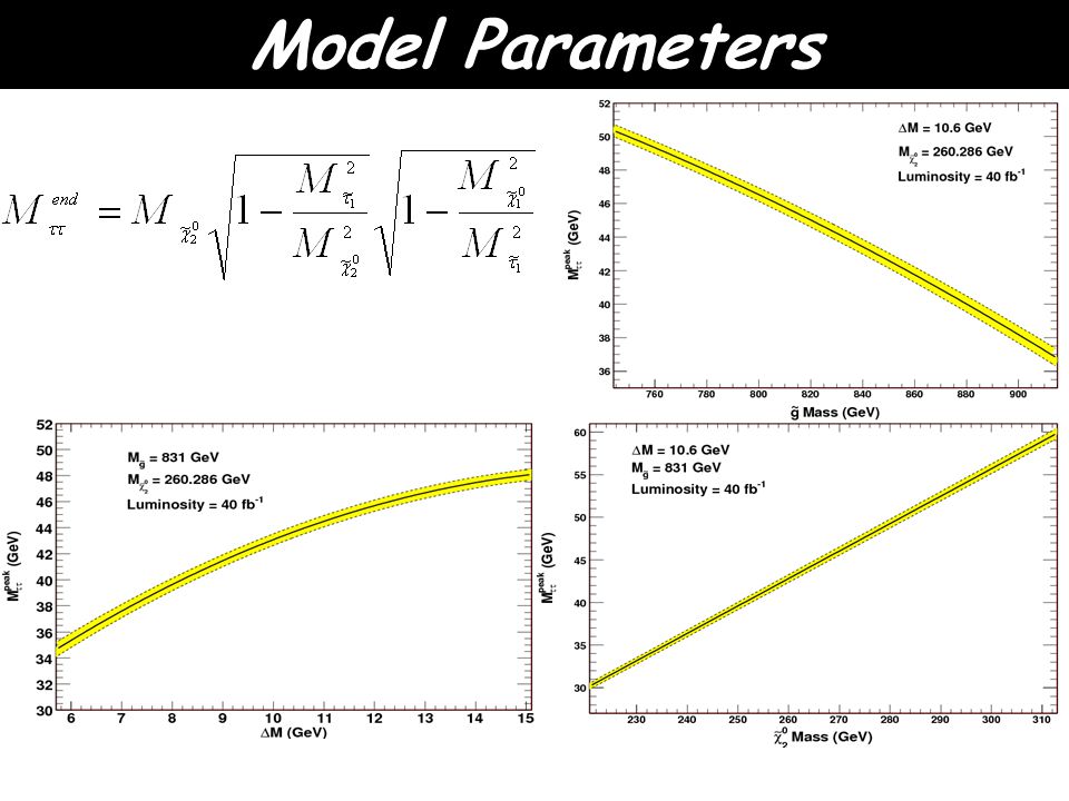
Can parameterize the our observables as functions of M,, & N OS-LS, to first order, does not depend on mass. A large increase or decrease in mass is needed to obtain a point that lies outside the error bars Cross-Section is dominated by the gluino mass Model Parameters

27
CONTOURS OF CONSTANT VALUES ( L = 40 fb -1 ) Intersection of the central contours provides the measurement of M,, & Auxilary lines determine the 1 region 1 st order test on Universality Testing Gaugino Universality
 Intersection of the central contours provides the measurement of M,, & Auxilary lines determine the 1 region 1 st order test on Universality Testing Gaugino Universality")
28
M and M gluino m 0 and m 1/2 (for fixed A 0 and tan We determine m 0 /m 0 ~ 1.2% and m 1/2 /m 1/2 ~2 % (for A 0 =0, tan =40) Determination of m 0 and m 1/2
 Determination of m 0 and m 1/2")
29
M and M gluino (for fixed A 0 and tan ) Determination of h 2 / h 2 ~ 7% (for A 0 =0, tan =40)
 Determination of h 2 / h 2 ~ 7% (for A 0 =0, tan =40)")
30
h 2 / h 2 ~ 7% for A 0 =0, tan =40 Analysis with visible E T > 20 GeV establishes stau- neutralino coannihilation region 2 analysis: Discovery with 10 fb 1 M / M ~ 5%, m g /m g ~ 2% using M peak, N OS-LS and p T The analyses can be done for the other models that don’t suppress 2 0 production. M eff will establish the existence of SUSY Different observables are needed to establish the dark matter allowed regions in SUSY model at the LHC Universality of gaugino masses can be checked Conclusion

Similar presentations

 Collaborators Satoru Kaneko,Takashi Shimomura, Masato Yamanaka,Oscar Vives Physical review D 78, 116013 (2008) arXiv:1002.????>")
 Majid Hashemi University of Antwerp, Belgium.>")

 30/5-3/6/2007 1 SM Background Contributions Revisited for SUSY DM Stau Analyses Based on 1.P. Bambade, M. Berggren,>")

>")
![June 8, 2007LPC Early CMS Physics1 Relic Density in MET+Jets+Taus Sample at the LHC Teruki Kamon Texas A&M University [1] Physics Case in MET+Jets+Taus.](/16/4919669/big_thumb.jpg "June 8, 2007LPC Early CMS Physics1 Relic Density in MET+Jets+Taus Sample at the LHC Teruki Kamon Texas A&M University [1] Physics Case in MET+Jets+Taus.>")


 on (1) Coannihilation, (2)>")


