1. Excel Graphing Tutorial Lauren Ottaviano Fall 2012

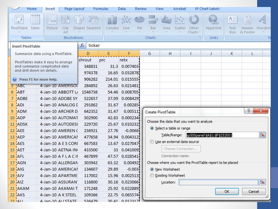
2. Pivot Tables For data that can be organized in multiple ways “Panel Data” E.g., multiple workers or companies –different years or days of data for each one. Makes it possible to slice and dice the data to create different summary statistics.

4. Pivot Tables

5. Right-click one of the variables in your field list to change it into a row label, a column label, or to make a summary statistic based upon it.

6. Pivot Tables “Calculated field” also makes it possible to add a new variable Like value = shares * price, for instance.

7. Graphs Select the cells that you want to graph E.g., two columns for a scatterplot A column of identifiers and column(s) of data for bar or column graphs. Go to Insert Tab & pick type of chart to make. Often a lot of reformatting is necessary to make things look nice.

10. Move chart  menu for where to place it Select “New Sheet”

11. Graphing Right click on a series to change the source data, line or fill colors, or to move some data to a secondary axis Drag & drop to move legends, axis titles Right click on axis to select “Format Axis”

12. Graphing Within axis options, it is possible to change the min & max values, where the tick marks appear, where one axis intersects the other, log scale, etc.

13. Graphing From the layout tab, it is possible to add axis titles, a legend, gridlines, a trend line, etc.

15. After some formatting...