2. Fiscal Policy CHAPTER 32

3. C H A P T E R C H E C K L I S T When you have completed your study of this chapter, you will be able to 1 Describe the federal budget process and the recent history of revenues, outlays, deficits, and debts. 2 Explain the supply-side effects of fiscal policy on employment and potential GDP. 3 Explain the demand-side effects of fiscal policy on employment and real GDP.

4. 32.1 THE FEDERAL BUDGET The federal budget is an annual statement of the revenues, outlays, and surplus or deficit of the government of the United States. The federal budget has two purposes: 1. To finance the activities of the federal government 2. To achieve macroeconomic objectives Fiscal policy is the use of the federal budget to achieve the macroeconomic objectives of high and sustained economic growth and full employment.

5. 32.1 THE FEDERAL BUDGET  The Institutions and Laws The President and the Congress make the budget and develop fiscal policy on a fixed annual time line and fiscal year. Fiscal year is a year that begins on October 1 and ends on September 30. Fiscal year 2008 begins in 2007.

7. 32.1 THE FEDERAL BUDGET  Budget Surplus or Budget Deficit Budget surplus (+)/deficit (–) = Tax revenues – Outlays The government has a budget surplus when tax revenues exceed outlays. The government has a budget deficit when outlays exceed tax revenues. The government has a balanced budget when tax revenues equal outlays.

8. 32.1 THE FEDERAL BUDGET  Surplus, Deficit, and Debt The government borrows to finance a budget deficit and repays its debt when it has a budget surplus. The amount of debt outstanding that arises from past budget deficits is called national debt. Debt at end of 2008 = Debt at end of 2007 + Budget deficit in 2008.

9. 32.1 THE FEDERAL BUDGET  The Federal Budget 2008

11. 32.2 THE SUPPLY SIDE AND POTENTIAL GDP Fiscal policy has important effects on potential GDP and aggregate supply. Supply-side effects are the effects of fiscal policy on potential GDP.

12. 32.2 THE SUPPLY SIDE AND POTENTIAL GDP  Fiscal Policy and Potential GDP Both sides of the government's budget influences potential GDP. The expenditure side provides public goods and services that enhance productivity. The increase in productivity increases potential GDP.

13. 32.2 THE SUPPLY SIDE AND POTENTIAL GDP On the revenue side, taxes modify incentives and change the equilibrium in the labor market and capital markets. An increase in taxes drives a wedge between the cost of labor to employers and the take-home pay of workers. Tax wedge in the labor market is the gap between the before-tax wage rate and the after-tax wage rate. The result is a decrease in the equilibrium quantity of labor employed and a decrease in potential GDP.

14. 32.2 THE SUPPLY SIDE AND POTENTIAL GDP  Fiscal Policy and Potential GDP: A Graphical Analysis Full Employment with No Income Tax The wage rate is $30 an hour and 250 billion hours of labor is employed.

15. 32.2 THE SUPPLY SIDE AND POTENTIAL GDP The economy is at full employment with 250 billion hours of labor employed. The production function shows that when 250 billion hours are employed, potential GDP is $11 trillion.

16. 32.2 THE SUPPLY SIDE AND POTENTIAL GDP The Effects of the Income Tax The income tax 1.Decreases the supply of labor. 2. Creates a tax wedge between the wage rate that firms pay and workers receive.

17. 32.2 THE SUPPLY SIDE AND POTENTIAL GDP 3.The before-tax wage rate rises to $35 an hour. 4.The after-tax wage rate falls to $20 an hour. 5.Full employment decreases to 200 billion hours.

19. 32.2 THE SUPPLY SIDE AND POTENTIAL GDP 5. Full employment decreases to 200 billion hours. 6. Potential GDP decreases to $10 trillion.

21. 32.2 THE SUPPLY SIDE AND POTENTIAL GDP  Taxes on Expenditure and the Tax Wedge Taxes on consumption expenditure add to the tax wedge that lowers potential GDP. The reason is that a tax on consumption expenditure raises the prices paid for consumption goods and services and is equivalent to a cut in the real wage rate. To find the total tax wedge, add the expenditure tax rate to the income tax rate. For example, if the income tax rate is 25 percent and the expenditure tax is 10 percent, the tax wedge is 35 percent.

22. 32.2 THE SUPPLY SIDE AND POTENTIAL GDP  Taxes, Deficits, and Economic Growth Fiscal policy influences economic growth in two ways: 1.Taxes drive a wedge between the interest rate paid by borrowers and the interest rate received by lenders. 2.If there is a budget deficit, government borrowing to finance the deficit competes with firms’ borrowing to finance investment and to some degree, government borrowing “crowds out” private investment.

23. 32.2 THE SUPPLY SIDE AND POTENTIAL GDP Interest Rate Tax Wedge Lenders pay an income tax on the interest they receive from borrowers, which creates an interest rate tax wedge. A tax on interest lowers the quantity of saving and investment and slows the growth rate of real GDP. A tax on interest income creates a Lucas wedge—an ever widening gap between potential GDP and the potential GDP that might have been.

24. 32.2 THE SUPPLY SIDE AND POTENTIAL GDP Investment and saving plans depend on the real after- tax interest rate. The real interest rate equals the nominal interest rate minus the inflation rate. So the after-tax interest rate equals the real interest rate minus the income tax paid on interest income. But the nominal interest rate, not the real interest rate, determines the amount of tax to be paid; and the higher the inflation rate, the higher is the nominal interest rate, and the higher is the true tax rate on interest income.

25. 32.2 THE SUPPLY SIDE AND POTENTIAL GDP Deficits and Crowding Out A tax cut that increases the budget deficit brings a decrease in the supply of loanable funds to firms. The interest rate rises and crowds out private investment. But the lower income tax rate shrinks the tax wedge and stimulates employment, saving, and investment. But a higher budget deficit lowers investment.

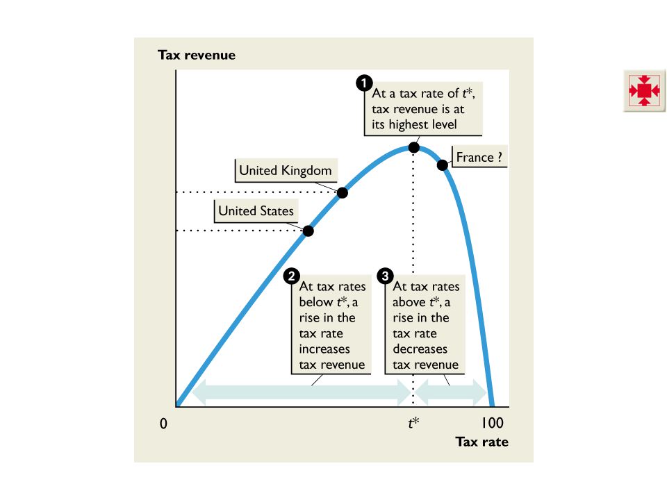
26. 32.2 THE SUPPLY SIDE AND POTENTIAL GDP  Income Tax Revenues and the Laffer Curve Laffer curve is the relationship between the tax rate and total tax revenue. As the tax rate rises, tax revenues rise, reach a maximum, and then fall. Figure 32.3 on the next slide illustrates the Laffer curve.

27. 32.2 THE SUPPLY SIDE AND POTENTIAL GDP 1. At a tax of t*, tax revenue is maximized. 2. For tax rates below t*, an increase in the tax rate increases tax revenue. For example, the United States and United kingdom. 3. For tax rates above t*, an increase in the tax rate decreases tax revenue. Perhaps France is an example.

29. 32.3 THE DEMAND SIDE: STABILIZING REAL GDP  Two Types of Fiscal Stabilizer Fiscal policy action that are aimed at stabilizing aggregate demand can be Discretionary fiscal policy Automatic fiscal policy

30. 32.3 THE DEMAND SIDE: STABILIZING REAL GDP Discretionary fiscal policy is a fiscal policy action that is initiated by an act of Congress. For example, an increase in defense spending or a cut in the income tax rate. Automatic fiscal policy is a fiscal policy action that is triggered by the state of the economy. For example, an increase in unemployment induces an increase in payments to the unemployed or in a recession tax receipts decrease as incomes fall.

31. 32.3 THE DEMAND SIDE: STABILIZING REAL GDP  Discretionary Fiscal Policy Multipliers The government expenditure multiplier is the magnification effect of a change in government expenditure on goods and services on aggregate demand. An increase in aggregate expenditure increases aggregate demand, which increases real GDP. The increase in real GDP induces an increase in consumption expenditure, which further increases aggregate demand.

32. 32.3 THE DEMAND SIDE: STABILIZING REAL GDP The Tax Multiplier The tax multiplier is the magnification effect of a change in taxes on aggregate demand. A decrease in taxes increases disposable income. The increase in disposable income increases consumption expenditure and aggregate demand. With increased aggregate demand, employment and real GDP increase and consumption expenditure increases yet further.

33. 32.3 THE DEMAND SIDE: STABILIZING REAL GDP So a decrease in taxes works like an increase in government expenditure. Both actions increase aggregate demand and have a multiplier effect. The magnitude of the tax multiplier is smaller than the government expenditure multiplier. The reason: A $1 tax cut increases aggregate expenditure by less than $1 whereas a $1 increase in government expenditure increases aggregate expenditure by $1.

34. 32.3 THE DEMAND SIDE: STABILIZING REAL GDP The Transfer Payments Multiplier The transfer payments multiplier is the magnification effect of a change in transfer payments on aggregate demand. This multiplier works like the tax multiplier but in the opposite direction. An increase in transfer payments increases disposable income, which increases consumption expenditure. With increased consumption expenditure, employment and real GDP increase and consumption expenditure increases yet further.

35. 32.3 THE DEMAND SIDE: STABILIZING REAL GDP The Balanced Budget Multiplier The balanced budget multiplier is the magnification effect on aggregate demand of a simultaneous change in government expenditure and taxes that leaves the budget balance unchanged. The balanced budget multiplier is not zero—it is positive—because the government expenditure multiplier is larger than the tax multiplier.

36. 32.3 THE DEMAND SIDE: STABILIZING REAL GDP  Expansionary Fiscal Policy If real GDP is below potential GDP, the government might use an expansionary fiscal policy in an attempt to restore full employment. Expansionary fiscal policy is a discretionary fiscal policy designed to increase aggregate demand—a discretionary increase in government expenditure or transfer payment or a discretionary tax cut.

37. 32.3 THE DEMAND SIDE: STABILIZING REAL GDP Potential GDP is $10 trillion, real GDP is $9 trillion, and 1. There is a $1 trillion recessionary gap. 2. An increase in government expenditure or a tax cut increases expenditure by ∆E. Figure 32.4 illustrates an expansionary fiscal policy.

38. 32.3 THE DEMAND SIDE: STABILIZING REAL GDP 3. The multiplier increases induced expenditure. The AD curve shifts rightward to AD 1. The price level rises to 110, real GDP increases to $10 trillion, and the recessionary gap is eliminated.

40. 32.3 THE DEMAND SIDE: STABILIZING REAL GDP  Contractionary Fiscal Policy If real GDP is above potential GDP, the government might use an contractionary fiscal policy in an attempt to restore full employment. Contractionary fiscal policy is a discretionary fiscal policy designed to decrease aggregate demand—a decrease in government expenditure, a decrease in transfer payment, or a tax increase.

41. 32.3 THE DEMAND SIDE: STABILIZING REAL GDP Figure 32.5 illustrates contractionary fiscal policy. Potential GDP is $10 trillion, real GDP is $11 trillion, and 1. There is a $1 trillion inflationary gap. 2. A decrease in government expenditure or a tax rise decreases expenditure by ∆E.

42. 32.3 THE DEMAND SIDE: STABILIZING REAL GDP 3. The multiplier decreases induced expenditure. The AD curve shifts leftward to AD 1. The price level falls to 110, real GDP decreases to $10 trillion, and the inflationary gap is eliminated.

44. 32.3 THE DEMAND SIDE: STABILIZING REAL GDP  Combined Demand-Side and Supply-Side Effects An increase in government expenditure or a tax cut increases equilibrium real GDP but might raise, lower, or have no effect on the price level. Figure 32.6 on the next slides shows the combined effects of fiscal policy when fiscal policy has no effect on the price level.

45. 32.3 THE DEMAND SIDE: STABILIZING REAL GDP 1. A tax cut increases disposable income, which increases aggregate demand from AD 0 to AD 1. A tax cut also strengthens the incentive to work, save, and invest, which increases aggregate supply from AS 0 to AS 1. 2. Real GDP increases.

47. 32.3 THE DEMAND SIDE: STABILIZING REAL GDP  Limitations of Discretionary Fiscal Policy The use of discretionary fiscal policy is seriously hampered by four factors: Law-making time lag Shrinking area of law-maker discretion Estimating potential GDP Economic forecasting

48. 32.3 THE DEMAND SIDE: STABILIZING REAL GDP Law-Making Time Lag The amount of time it takes Congress to pass the laws needed to change taxes or spending. This process takes time because each member of Congress has a different idea about what is the best tax or spending program to change, so long debates and committee meetings are needed to reconcile conflicting views.

49. 32.3 THE DEMAND SIDE: STABILIZING REAL GDP Shrinking Area of Law-Maker Discretion Expenditure on the military and on homeland security and very large expansion in expenditure on entitlement programs such as Medicare has increased. The result is that around 80 percent of the federal budget is effectively off limits for discretionary fiscal policy action. The 20 percent that is available for discretionary change include items such as education and the space program, which are very hard to cut.

50. 32.3 THE DEMAND SIDE: STABILIZING REAL GDP Estimating Potential GDP It is not easy to tell whether real GDP is below, above, or at potential GDP. So a discretionary fiscal action might move real GDP away from potential GDP instead of toward it. This problem is a serious one because too much fiscal stimulation brings inflation and too little might bring recession.

51. 32.3 THE DEMAND SIDE: STABILIZING REAL GDP Economic Forecasting Fiscal policy changes take a long time to enact in Congress and yet more time to become effective. So fiscal policy must target forecasts of where the economy will be in the future. Economic forecasting has improved enormously in recent years, but it remains inexact and subject to error. So for a second reason, discretionary fiscal action might move real GDP away from potential GDP and create the very problems it seeks to correct.

52. 32.3 THE DEMAND SIDE: STABILIZING REAL GDP  Automatic Fiscal Policy A consequence of tax receipts and expenditures that fluctuate with real GDP. Automatic stabilizers are features of fiscal policy that stabilize real GDP without explicit action by the government. Induced Taxes Induced taxes are taxes that vary with real GDP.

53. 32.3 THE DEMAND SIDE: STABILIZING REAL GDP Needs-Tested Spending Needs-tested spending is spending on programs that entitle suitably qualified people and businesses to receive benefits— benefits that vary with need and with the state of the economy.