Download presentation
Presentation is loading. Please wait.

1
Watershed Management Runoff models
Hydrology and Water Resources, RG744 Institute of Space Technology November 13, 2013

2
Runoff models Peak runoff models Continuous runoff models
Provide only the estimates of peak discharge from the watershed Continuous runoff models This class of runoff models provides storm hydrographs for a given rainfall hyetograph Provide an estimate of runoff vs. time series

3
Peak runoff models Rational Method NRCS Method

4
Rational Method To calculate peak runoff from small watersheds
Provides peak runoff rate from a catchment given: the runoff coefficient C, the time of concentration Tc, the area of the catchment, and the information to calculate the input or design storm or rainfall event Also called Lloyd Davies Method, 1850 Source: The McGraw-Hill civil engineering PE exam depth guide: water resources By Emmanuel U. Nzewi

5
Rational Method: Assumptions
Catchment is small (less than 200 acres) Catchment is concentrated Rainfall intensity is uniform over the area of study The runoff coefficient is catch-all coefficient that incorporates all losses of the catchment Source: The McGraw-Hill civil engineering PE exam depth guide: water resources By Emmanuel U. Nzewi. Catchment is concentrated: that is, rainfall duration is longer than or at least equal to the time of concentration of the watershed.
 Catchment is concentrated. Rainfall intensity is uniform over the area of study. The runoff coefficient is catch-all coefficient that incorporates all losses of the catchment. Source: The McGraw-Hill civil engineering PE exam depth guide: water resources By Emmanuel U. Nzewi. Catchment is concentrated: that is, rainfall duration is longer than or at least equal to the time of concentration of the watershed.")
6
Rational method: formula
Qp = CIiA Qp = Peak discharge (cfs) C = runoff coefficient (function of soil type and drainage basin slope) Ii = average rainfall intensity (in/hr) for a storm duration equal to the time of concentration, Tc A = area (acre) For runoff coefficient refer Bedient Table 6-5 page 381 Obtain i from IDF curve with tr (duration) and T defined (assume tr = Tc) C = runoff coefficient, ratio of the total runoff rate to the precipitation, dimensionless
 C = runoff coefficient (function of soil type and drainage basin slope) Ii = average rainfall intensity (in/hr) for a storm duration equal to the time of concentration, Tc. A = area (acre) For runoff coefficient refer Bedient Table 6-5 page 381. Obtain i from IDF curve with tr (duration) and T defined (assume tr = Tc) C = runoff coefficient, ratio of the total runoff rate to the precipitation, dimensionless.")
7
Determining Tc Take Tc = 5min when A (acres) < 4.6 S (slope %)
Or use Kinematic Wave Theory (iterative process) L = length of overland flow plane (feet) S = slope (ft/ft) n = Manning roughness Ii= Rainfall intensity (in/hr) C = rational runoff coefficient Source:
 L = length of overland flow plane (feet) S = slope (ft/ft) n = Manning roughness. Ii= Rainfall intensity (in/hr) C = rational runoff coefficient. Source:")
8
Rational Method: example 6-6 Bedient
Drainage design to be accomplished for a 4 acre asphalt parking lot in Tallahassee for a 5 yr return period. The dimensions are such that the overland flow length is 1000 ft down a 1% slope. What will be the peak runoff rate? Refer Table 6-5, 4-2 & Figure 6-5 Assume tr value, for that value read rainfall intensity from IDF curve. Calculate Tc using Kinematic wave theory. (iterate till tr = Tc) Page 383
 Page 383.")
9
Runoff coefficient for nonhomogeneous area
Weighted runoff coefficient based on area of each land use Cw = ∑j=1 n Cj Aj/ ∑j=1 n Aj Example McCuen page 381 C reflects the effect of landuse, soil and slope on runoff potential assuming watershed is homogeneous. If drainage basin has different runoff potentials then it’s subdivided.

10
November 20, 2013

11
NRCS Runoff Curve Number Methods
By the USA Soil Conservation Service (now called the Natural Resources Conservation Service), division of the USDA (USA Department of Agriculture) To predict peak discharge due to a 24-hr storm event Empirically derived relationships that use precipitation, land cover and physical characteristics of watershed to calculate runoff amount, peak discharges and hydrographs More sophisticated approach than Rational Method Source: National Resources Conservation Service (NRCS) (formally SCS) The RCN (Runoff Curve Number) method was originally established by the SCS in 1954. Initially developed as a design tool to estimate runoff from rainfall events on Agricultural fields. Now used for computing peak runoff rates and volumes for Urban Hydrology. Note: TR (Technical Release) -55 a simplified NRCS tool essentially joins the NRCS runoff equation with unit hydrograph theory for the computation of these runoff rates.
, division of the USDA (USA Department of Agriculture) To predict peak discharge due to a 24-hr storm event. Empirically derived relationships that use precipitation, land cover and physical characteristics of watershed to calculate runoff amount, peak discharges and hydrographs. More sophisticated approach than Rational Method. Source: National Resources Conservation Service (NRCS) (formally SCS) The RCN (Runoff Curve Number) method was originally established by the SCS in Initially developed as a design tool to estimate runoff from rainfall events on Agricultural fields. Now used for computing peak runoff rates and volumes for Urban Hydrology. Note: TR (Technical Release) -55 a simplified NRCS tool essentially joins the NRCS runoff equation with unit hydrograph theory for the computation of these runoff rates.")
12
NRCS Curve number Curve number is a coefficient that reduces the total precipitation to runoff potential, after “losses” Evaporation Absorption Transpiration Surface Storage Higher the CN value - higher the runoff potential will be It is essential to use the CN value that best mimics the Ground Cover Type and Hydrologic Condition

13
NRCS Rainfall-Runoff Equation
Following equation presents relationship between accumulated rainfall and accumulated runoff Where: Q = accumulated direct runoff (in. or mm) P = accumulated rainfall (potential maximum runoff) (in. or mm) (24-Hour Rainfall Depth versus Frequency Values) Ia = initial abstraction including surface storage, interception, evaporation and infiltration prior to any runoff occurring (in. or mm) S = potential maximum soil moisture retention after runoff begins (in. or mm) Note: for P ≤ Ia, Q = 0 Equation 1 Eq-1 Derived by NRCS from experimental plots for numerous soils and vegetative cover conditions. The simplified NRCS method can be used for drainage areas up to 2,000 acres. Ia is highly variable, but generally is correlated with soil and landcover parameters. Through studies of many small agricultural watersheds, Ia was found to be approximated by the following empirical equation: Ia = 0.2S. S is related to the soil and cover conditions of the watershed through the curve number, CN (0-100 range). If P- Ia is negative then Q=0
 P = accumulated rainfall (potential maximum runoff) (in. or mm) (24-Hour Rainfall Depth versus Frequency Values) Ia = initial abstraction including surface storage, interception, evaporation and infiltration prior to any runoff occurring (in. or mm) S = potential maximum soil moisture retention after runoff begins (in. or mm) Note: for P ≤ Ia, Q = 0. Equation 1. Eq-1 Derived by NRCS from experimental plots for numerous soils and vegetative cover conditions. The simplified NRCS method can be used for drainage areas up to 2,000 acres. Ia is highly variable, but generally is correlated with soil and landcover parameters. Through studies of many small agricultural watersheds, Ia was found to be approximated by the following empirical equation: Ia = 0.2S. S is related to the soil and cover conditions of the watershed through the curve number, CN (0-100 range). If P- Ia is negative then Q=0.")
14
potential maximum retention (S)
potential maximum retention (S) can be calculated using Equation 2 Where: z=10 for English measurement units, or 254 for metric CN = Runoff Curve Number Generally, Ia may be estimated as Ia = 0.2 S Equation 3 Substituting Ia value in Equation 1 Equation 2 Equation 2 was developed mainly for small watersheds from recorded storm data that included total rainfall amount in a calendar day but not its distribution with respect to time. Therefore, this method is appropriate for estimating direct runoff from 24-hour or one-day storm rainfall Equation 4
 can be calculated using Equation 2. Where: z=10 for English measurement units, or 254 for metric. CN = Runoff Curve Number. Generally, Ia may be estimated as. Ia = 0.2 S Equation 3. Substituting Ia value in Equation 1. Equation 2. Equation 2 was developed mainly for small watersheds from recorded storm data that included total rainfall amount in a calendar day but not its distribution with respect to time. Therefore, this method is appropriate for estimating direct runoff from 24-hour or one-day storm rainfall. Equation 4.")
15
NRCS Runoff equations Source:

16
Estimation of CN Equation 4 (slide# 14) can be rearranged so the CN can be estimated if rainfall and runoff volume are known (Pitt, 1994) The equation then becomes: Source:

17
Note: The initial Abstraction is greater than or equal to the Rainfall for values to the left of the red line. Table Source:

18
Series of curve for different curve numbers

19
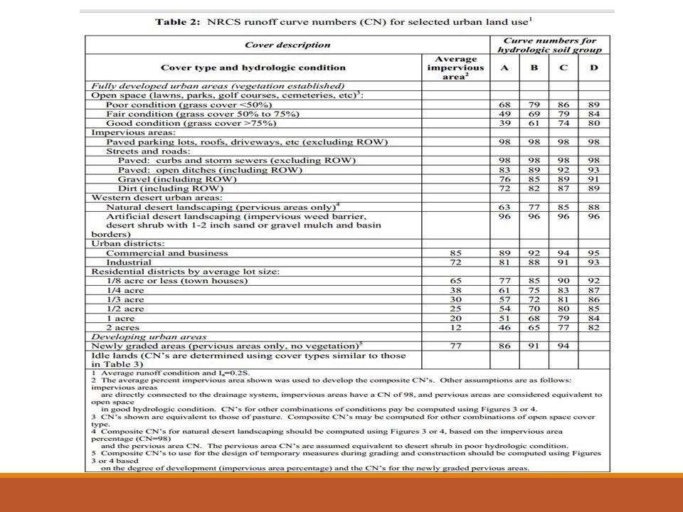
Curve Number CN The principal physical watershed characteristics affecting the relationship between rainfall and runoff are land use, land treatment, soil types, and land slope. NRCS method uses a combination of soil conditions and land uses (ground cover) to assign a runoff factor to an area (CN) CN indicates the runoff potential of an area Higher the CN, the higher the runoff potential Soil properties also influence the relationship between runoff and rainfall since soils have differing rates of infiltration Based on infiltration rates, the NRCS has divided soils into four hydrologic soil groups
 to assign a runoff factor to an area (CN) CN indicates the runoff potential of an area. Higher the CN, the higher the runoff potential. Soil properties also influence the relationship between runoff and rainfall since soils have differing rates of infiltration. Based on infiltration rates, the NRCS has divided soils into four hydrologic soil groups.")
20
Composite Curve Number
When a drainage area has more than one land use When Composite CN is used Analysis does not take into account the location of the specific land uses drainage area is considered as a uniform land use represented by the composite curve number can be calculated by using the weighted method

21
Hydrologic Soil groups
Hydrologic Group is a grouping of soils that have similar runoff potential under similar storm and cover conditions Group A Soils: High infiltration (low runoff). Sand, loamy sand, or sandy loam. Infiltration rate > 0.3 inch/hr when wet. Group B Soils: Moderate infiltration (moderate runoff). Silt loam or loam. Infiltration rate 0.15 to 0.3 inch/hr when wet. Group C Soils: Low infiltration (moderate to high runoff). Sandy clay loam. Infiltration rate 0.05 to 0.15 inch/hr when wet. Group D Soils: Very low infiltration (high runoff). Clay loam, silty clay loam, sandy clay, silty clay, or clay. Infiltration rate 0 to 0.05 inch/hr when wet. Effects of Urbanization: Consider the effects of urbanization on the natural hydrologic soil group. If heavy equipment can be expected to compact the soil during construction or if grading will mix the surface and subsurface soils, you should make appropriate changes in the soil group selected. Antecedent soil moisture conditions: AMC I, II and III Average antecedent soil moisture conditions (AMC II) are recommended for most hydrologic analysis
. Sand, loamy sand, or sandy loam. Infiltration rate > 0.3 inch/hr when wet. Group B Soils: Moderate infiltration (moderate runoff). Silt loam or loam. Infiltration rate 0.15 to 0.3 inch/hr when wet. Group C Soils: Low infiltration (moderate to high runoff). Sandy clay loam. Infiltration rate 0.05 to 0.15 inch/hr when wet. Group D Soils: Very low infiltration (high runoff). Clay loam, silty clay loam, sandy clay, silty clay, or clay. Infiltration rate 0 to 0.05 inch/hr when wet. Effects of Urbanization: Consider the effects of urbanization on the natural hydrologic soil group. If heavy equipment can be expected to compact the soil during construction or if grading will mix the surface and subsurface soils, you should make appropriate changes in the soil group selected. Antecedent soil moisture conditions: AMC I, II and III. Average antecedent soil moisture conditions (AMC II) are recommended for most hydrologic analysis.")
22
Antecedent soil moisture conditions-AMC
AMC is the preceding relative moisture of the pervious surfaces prior to the rainfall event Low: when there has been little preceding rainfall High: when there has been considerable preceding rainfall prior to the modeled rainfall event ACM I (dry), ACM II (average) and ACM III (wet) For modeling purposes, we consider watersheds to be AMC II, which is essentially an average moisture condition also referred to as Antecedent Runoff Condition (ARC).
, ACM II (average) and ACM III (wet) For modeling purposes, we consider watersheds to be AMC II, which is essentially an average moisture condition. also referred to as Antecedent Runoff Condition (ARC).")
23
CNs A CN of 100 is to be used for permanent water surfaces such as lakes and ponds

24
http://www. ctre. iastate
27
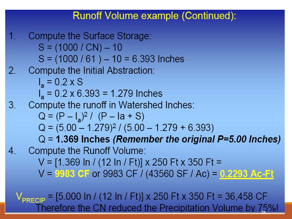
Example Source:

29
Continuous Runoff Models
Time area method Unit Hydrograph Techniques Source: The McGraw-Hill civil engineering PE exam guide: breadth and depth By Roger Dodge Woodson, Kimberly Griffin.

30
Time Area Method Develop to address non-uniform rainfall in large areas Convert rainfall excess into hydrograph Concept of time-area histogram is used This method assumes that outflow hydrograph results from pure translation of direct runoff to the outlet at uniform velocity, ignoring any storage effects in the watershed Watershed divided into subareas with distinct runoff translation times to the outlet Subareas are delineated with isochrones of equal translation time (numbered upstream from the outlet) Source: Bedient page 111
 Source: Bedient page 111.")
31
Time Area Method If a rainfall of uniform intensity is distributed over the watershed area, water first flows from are as immediately adjacent to the outlet Percentage of the total area contributing increases progressively in time Example : Surface runoff from area A1 will reach the outlet first, followed by contributions from A2, A3, …..and so on Qn = RiA1+Ri-1A2+…….R1Aj Qn = Hydraulic ordinate at time n (cfs) Ri= excess rainfall ordinate at time i (ft/s) Aj= time-area histogram ordinate at time j (ft2)
 Ri= excess rainfall ordinate at time i (ft/s) Aj= time-area histogram ordinate at time j (ft2)")
32
Isochrones: a line on a map or diagram connecting places from which it takes the same time to travel to a certain point. Isochrones of equal translation time numbered upstream from the outlet Source:

33
Example 2-2 from Bedient page 112
Time area histogram method. The following is an example of the inflow for hour 5 using the 5 hour rainfall and 4 sub-basins. Assume constant rainfall intensity of 0.5in/hr

34
November 27, 2013

35
Unit Hydrograph (UHG) Theory
Unit Hydrograph of a watershed is defined as the direct runoff hydrograph resulting from a unit depth of rainfall excess (1 in or 1 cm) distributed uniformly over a drainage area at a constant rate for an effective duration The effective rainfall is considered uniformly distributed within its duration and throughout the whole area of the basin Uniquely represents storm-flow response (hydrograph shape) for a given watershed Time area method is a special case of the unit hydrograph method. Introduced by Sherman in 1932 1 cm in SI units To be applied only to direct runoff.
 distributed uniformly over a drainage area at a constant rate for an effective duration. The effective rainfall is considered uniformly distributed within its duration and throughout the whole area of the basin. Uniquely represents storm-flow response (hydrograph shape) for a given watershed. Time area method is a special case of the unit hydrograph method. Introduced by Sherman in cm in SI units. To be applied only to direct runoff.")
36
Unit Hydrograph Theory: Assumptions
The effective rainfall is uniformly distributed within its duration The effective rainfall is uniformly distributed throughout the whole area of the basin The base period of the direct runoff hydrograph produced by effective rainfall of same duration (intensities may be different) are also same The ordinates of the direct runoff hydrographs of a common base period are directly proportional to the total volume of direct runoff represented by the respective hydrographs For a given drainage basin the hydrograph of runoff due to a given period of rainfall reflects the unchanging characteristics of the basin Source: A Textbook of Hydrology By P. Jaya Rami Reddy If there are N number of rain gages spread uniformly over the basin, then all gages should record almost same amount of rainfall during the specified period. 1 & 2 incorporated in definition of UHG, 4 is linearity principle, 3 and 5 imply that shape of runoff hydrograph remains same irrespective of time it occurs as long as the duration of rainfall producing it is same.
 are also same. The ordinates of the direct runoff hydrographs of a common base period are directly proportional to the total volume of direct runoff represented by the respective hydrographs. For a given drainage basin the hydrograph of runoff due to a given period of rainfall reflects the unchanging characteristics of the basin. Source: A Textbook of Hydrology By P. Jaya Rami Reddy. If there are N number of rain gages spread uniformly over the basin, then all gages should record almost same amount of rainfall during the specified period. 1 & 2 incorporated in definition of UHG, 4 is linearity principle, 3 and 5 imply that shape of runoff hydrograph remains same irrespective of time it occurs as long as the duration of rainfall producing it is same.")
37
Unit Hydrograph Theory: Assumptions
2 Basic Assumptions: Time Invariance Direct runoff response to a given effective rainfall in a catchment is time invariant, i.e. direct-runoff hydrograph (DRH) for a given excess rainfall in a catchment is always the same irrespective of when it occurs Linear Response Direct runoff response to the rainfall excess is assumed to be linear. Means if inputs x1(t), x2(t) cause outputs y1(t) and y2(t) respectively then an input x1(t) + x2(t) will cause an output y1(t) + y2(t). Also if x1(t) = r x2(t) then y1(t) = r y2(t). Source: A Textbook of Hydrology By P. Jaya Rami Reddy????
 for a given excess rainfall in a catchment is always the same irrespective of when it occurs. Linear Response. Direct runoff response to the rainfall excess is assumed to be linear. Means if inputs x1(t), x2(t) cause outputs y1(t) and y2(t) respectively then an input x1(t) + x2(t) will cause an output y1(t) + y2(t). Also if x1(t) = r x2(t) then y1(t) = r y2(t). Source: A Textbook of Hydrology By P. Jaya Rami Reddy")
38
Linear Response Source: usf ( tp= time to peak from start of rainfall UH is 1/2 the size but TB (time base) and TP (time to peak) are the same
 and TP (time to peak) are the same.")
39
Typical Unit Hydrograph
Source: Engineering Hydrology By K. Subramanya Runoff volume = meter cube Direct runoff = 1 cm Runoff volume= Catchment area x direct runoff Catchment area = Runoff volume/direct runoff = 1292 square km

40
Properties of unit hydrograph
Volume under unit hydrograph is equal to 1 unit rainfall excess (1 in or cm) If duration of 2 rainfall excess events is equal without regard to their respective rainfall intensities, they must result in the same hydrograph time base Results in a linear system whereby the direct runoff for storm of specified duration is directly proportional to the rainfall excess amount or volume Rainfall distribution for all equal duration storms is identical in time and space Source: The McGraw-Hill civil engineering PE exam guide: breadth and depth By Roger Dodge Woodson, Kimberly Griffin.
 If duration of 2 rainfall excess events is equal without regard to their respective rainfall intensities, they must result in the same hydrograph time base. Results in a linear system whereby the direct runoff for storm of specified duration is directly proportional to the rainfall excess amount or volume. Rainfall distribution for all equal duration storms is identical in time and space. Source: The McGraw-Hill civil engineering PE exam guide: breadth and depth By Roger Dodge Woodson, Kimberly Griffin.")
41
Development of UHG Examine records of watershed for single peaked, isolated stream flow hydrographs resulting from short duration rainfall hyetograph of relatively uniform intensity Determine depth of storm precipitation spread over the watershed equivalent to the volume of water divided by area Volume is equal to area under hydrograph Ordinates of UHG can be calculated by dividing the ordinates of the DRH by the storm depth Check: recalculate area under UHG and divide it by watershed area. That should give unit storm depth. Source: Brooks pg 444

42
Example: Determine the UHG ordinates for the hydrograph shown in figure. The area of watershed is 16.2 square km Source: Intro To Env Engg (Sie), 4E By Davis
, 4E By Davis.")
43
= 0.5 (m cube/sec) * 1hr (60x60 sec/hr) = 1,800 m cube
 * 1hr (60x60 sec/hr) = 1,800 m cube")
44
Source: Intro to Env Engg by Davis

45
Example Source: Engineering Hydrology By Subramanya

46
Table:

47
3.5 cm Direct Runoff Hydrograph

48
Drg ordinates from uhg with Variable Rainfall excess values (M pulses of excess rainfall
Discrete Convolution Equation is used to compute direct runoff hydrograph ordinates Qn = direct runoff hydrograph ordinates, Pm= Rainfall excess, Un-m+1 = unit hydrograph ordinates, n= direct runoff hydrograph time interval (1, 2, …N), m= precipitation time interval M = pulses of excess of rainfall N = pulses of direct runoff N-M+1 = L, Number of UH ordinates Reverse process is called ‘deconvolution’ to derive unit hydrograph given Pm and Qn Source: Water Resources Engineering By Larry W. Mays
, m= precipitation time interval. M = pulses of excess of rainfall. N = pulses of direct runoff. N-M+1 = L, Number of UH ordinates. Reverse process is called ‘deconvolution’ to derive unit hydrograph given Pm and Qn. Source: Water Resources Engineering By Larry W. Mays.")
49
Discrete time convolution equations

50
Application of uhg to rainfall input

51
Deconvolution process
Q n and Pm are known Q1 = P1 * U1 (Q1 and P1 known, calculate U1) Q2= P2*U1 + P1 *U2 (all known except U2) And so on Source: A Textbook of Hydrology By P. Jaya Rami Reddy
 Q2= P2*U1 + P1 *U2 (all known except U2) And so on. Source: A Textbook of Hydrology By P. Jaya Rami Reddy.")
52
Example: Source: Water Resources Engineering By Larry W. Mays (Google Book)
")
53
Example Hard copies provided in class
Reading material on Hydrograph Analysis:

54
December 11, 2013

55
Instantaneous Unit Hydrograph
Limiting the duration of UHG to zero an Instantaneous Unit Hydrograph is obtained Instantaneous Unit Hydrograph is the hydrograph resulting from an instantaneous rainfall of one unit uniformly over the basin UHG depends on duration of excess rainfall (disadvantage).
.")
56
Synthetic UHG When observed rainfall/runoff data for a catchment is not available to derive UHG Construct synthetic UHG based on empirical functions (basin’s physical characteristics) Developing UHG for other locations on the stream in the same watershed or other watersheds that are of similar character with known data Snyder’s Unit Hydrograph SCS Dimensionless Unit Hydrograph Clark (time area method)
 Developing UHG for other locations on the stream in the same watershed or other watersheds that are of similar character with known data. Snyder’s Unit Hydrograph. SCS Dimensionless Unit Hydrograph. Clark (time area method)")
57
Snyder UHG Relates the time from the centroid of the rainfall to the peak of the UHG to geometrical characteristics of the watershed Important factors to be considered for a UGH are; peak flow and time of peak flow Coefficient derived from gaged watershed in the area Cp and Ct Cp = peak flow factor, and Ct = lag factor. Basic Assumption of Synder’s Method: that basins which have similar physiographic characteristics are located in the same area will have similar values of Cp and Ct Therefore, for ungagged basins, it is preferred that the basin be near or similar to gaged basins for which these coefficients can be determined Water Resources Engineering By Larry W. Mays Source: Ct = represents variation in watershed slopes and storage characteristics. Cp = represents the effect of retention and storage.

58
Snyder’s UHG: Computing Ct
tp = basin lag time (hrs) Lc= distance from outlet to a point on the stream nearest the centroid of the watershed area -in km (miles) L = length of main stream from outlet to the upstream divide - in km (miles) C1 = 0.75 ( 1.0 for English units) 𝐶𝑡= 𝑡𝑝 𝐶1 𝐿.𝐿𝑐 0.3 L Lc = measure of watershed shape. L and Lc are determined from gaged watershed and tp from derived unit hydrograph for the gaged basin.
 Lc= distance from outlet to a point on the stream nearest the centroid of the watershed area -in km (miles) L = length of main stream from outlet to the upstream divide - in km (miles) C1 = 0.75 ( 1.0 for English units) 𝐶𝑡= 𝑡𝑝 𝐶1 𝐿.𝐿𝑐 0.3. L Lc = measure of watershed shape. L and Lc are determined from gaged watershed and tp from derived unit hydrograph for the gaged basin.")
59
Snyder’s UHG: Computing Cp
Qp = peak direct runoff rate - in m3/s (cfs) A = watershed area - in km2 (mi2), qp= peak discharge/unit watershed area C2 = 2.75 (640 for English units) 𝑄𝑝= 𝐴 𝐶2𝐶𝑝 𝑡𝑝 Or for a unit discharge (discharge per unit area) 𝑞𝑝= 𝐶2𝐶𝑝 𝑡𝑝 Or 𝐶𝑝= 𝑞𝑝𝑡𝑝 𝐶2 English units (ft)
 A = watershed area - in km2 (mi2), qp= peak discharge/unit watershed area. C2 = 2.75 (640 for English units) 𝑄𝑝= 𝐴 𝐶2𝐶𝑝 𝑡𝑝. Or for a unit discharge (discharge per unit area) 𝑞𝑝= 𝐶2𝐶𝑝 𝑡𝑝. Or. 𝐶𝑝= 𝑞𝑝𝑡𝑝 𝐶2. English units (ft)")
60
Characteristics of a Standard UHG
tp = 5.5 tr tp = C1Ct (LLc) 𝑄𝑝= 𝐴 𝐶2𝐶𝑝 𝑡𝑝 tp = basin lag – time from the centroid of excess rainfall hyetograph to the peak runoff (hrs) Qp = peak direct runoff rate
 𝑄𝑝= 𝐴 𝐶2𝐶𝑝 𝑡𝑝 tp = basin lag – time from the centroid of excess rainfall hyetograph to the peak runoff (hrs) Qp = peak direct runoff rate.")
62
Snyder: Development of a Required UHG
assuming that Ct, Cp, L, and Lc are known Required: a unit hydrograph whose associated effective rainfall pulse duration is tR for an ungagged watershed Use equation 2 to determine the lag-time, tp If tR meets the criterion for a standard UHG (tp = 5.5 tR) then the required unit hydrograph is a standard UHG equations 2 and 3 can be used directly to estimate the peak discharge and the time to peak of the required unit hydrograph If tR does not meet the criterion for a standard UHG In this case, the lag-time of the required unit hydrograph, tpR, is tpR = tp – (tr – tR)/ where tp is obtained from equation 2, tr is obtained from equation 1 and tR is given. Source: Snyder’s UHG
 then the required unit hydrograph is a standard UHG. equations 2 and 3 can be used directly to estimate the peak discharge and the time to peak of the required unit hydrograph. If tR does not meet the criterion for a standard UHG. In this case, the lag-time of the required unit hydrograph, tpR, is. tpR = tp – (tr – tR)/ where tp is obtained from equation 2, tr is obtained from equation 1 and tR is given. Source: Snyder’s UHG.")
63
Conti… The peak discharge of the required UHG, QpR, is,
QpR = Qp tp/tpR where Qp is obtained from equation 3 Assuming a triangular shape for the UHG, and given that the UHG represents a direct runoff volume of 1 cm (1 in), the base time of the required UHG may be estimated by tb = C3A/QpR where C3 is 5.56 (1290 for the English system)
, the base time of the required UHG may be estimated by. tb = C3A/QpR where C3 is 5.56 (1290 for the English system)")
64
Drawing Snyder’s UHG Relationships for the widths of the UHG at values of 50% (W50) and 75% (W75) of QpR developed by U.S. Army Corps of Engineers; W% = Cw(QpR/A)-1.08 where the constant Cw is 1.22 (440 for English units) for the 75% width and equals to 2.14 (770 for English units) for the 50% width
 where the constant Cw is 1.22 (440 for English units) for the 75% width and equals to 2.14 (770 for English units) for the 50% width.")
65
Snyder’s Synthetic UHG
Source:

66
Example: Snyder’s Method
A watershed has a drainage area of 5.42 mi2; length of the main stream is 4.45 mi, and the main channel length from the watershed outlet to the point opposite the center of gravity of the watershed is 2.0 mi, Using Ct = 2.0 and Cp = 0.625, determine the standard synthetic UHG for this basin. What is the standard duration? Use Snyder’s method to determine 30 min unit hydrograph parameters. Solution: Given: Ct = 2.0, Cp = 0.625, Lc = 2.0 mi, L= 4.45 mi, tR= 30 mi (0.5 hr), C1 = 1, C2 = 640, C3 = 1290 Equation tp = C1 Ct (LLc)0.3 =1 x2 (4.45 x 2) 0.3 = 3.85 hrs Equation Standard rainfall duration, tr = tp/5.5 = 3.85/5.5 = 0.7 hrs, tr ≠ tR. Equation tpR = tp – (tr – tR)/4 = 3.85 – (0.7 – 0.5)/4 = 3.8 hrs Equation 𝑄𝑝= 𝐴 𝐶2𝐶𝑝 𝑡𝑝 = 5.42 x 640 x 0.625/3.85 = 563 cfs Equation QpR = Qp tp/tpR = 563 x 3.85/3.8 = cfs Equation tb = C3A/QpR = 1290 x 5.42 /570.5 = hrs Example pg#295, Water Resources Engineering By Larry W. Mays
, C1 = 1, C2 = 640, C3 = Equation tp = C1 Ct (LLc)0.3 =1 x2 (4.45 x 2) 0.3 = 3.85 hrs. Equation Standard rainfall duration, tr = tp/5.5 = 3.85/5.5 = 0.7 hrs, tr ≠ tR. Equation tpR = tp – (tr – tR)/4 = 3.85 – (0.7 – 0.5)/4 = 3.8 hrs. Equation 𝑄𝑝= 𝐴 𝐶2𝐶𝑝 𝑡𝑝 = 5.42 x 640 x 0.625/3.85 = 563 cfs. Equation QpR = Qp tp/tpR = 563 x 3.85/3.8 = cfs. Equation tb = C3A/QpR = 1290 x 5.42 /570.5 = hrs. Example pg#295, Water Resources Engineering By Larry W. Mays.")
67
SCS unit hydrograph Slide source: 484 = 2/2.67 *(5280 ft/mi x 5280 ft/mi) x 1/12 (ft/in) x 1/3600 (hr/sec) = cfs
 x 1/12 (ft/in) x 1/3600 (hr/sec) = cfs.")
68
Clark’s IUH Time-Area Method (concept of isochrones)
Slide source: Isochrones are lines of equal travel time. Any point on a given isochrone takes the same time to reach the basin outlet.

69
HYDROGRAPHS Floods 2013 in Sindh
Map layout prepared by M. Arslan student MS-5 batch at RS and GISc, IST Karachi Campus. HYDROGRAPHS Floods 2013 in Sindh

70
Source: SIDA: http://www.sida.org.pk/pages.aspx?id=82

Similar presentations


>")
 Synthetic unit hydrographs>")
>")


 How many.>")
