1. The Normal Curve

2. Probability Distribution Imagine that you rolled a pair of dice. What is the probability of 5-1? To answer such questions, we need to compute the whole population for possible results of rolling two dices. A standard dice has six faces. The probability of a number on a dice is 1/6.

3. Probability Distribution We have two unrelated populations. That is, the results of the dices are not dependent. So, the probability of 5-1 is equal to 1/6 * 1/6 = 1/36. That means, in the perfect universe of math, if we roll two dice for 36 times, than one of the results will be 5-1. We can see that in the table below

4. Probability Distribution 1-11-21-31-41-51-6 2-12-22-32-42-52-6 3-13-23-33-43-53-6 4-14-24-34-44-54-6 5-15-25-35-45-55-6 6-16-26-36-46-56-6 So, the probability of 5 – 1 is 1/36. But remember, it is the probability of the event that the first dice (and only the first one) will be 5 and the second one will be 1

5. Probability Distribution What if we would like to find the probability of the number 6 in that table? – That is the events when the sum of the two dices will be six. Which combinations of two dices produce the score 6? – Let’s see in the same table

6. Probability Distribution So, the probability of the score 6 is 5/36. That is, in the perfect conditions 5 of 36 trails will result in the score 6. 1-11-21-31-41-51-6 2-12-22-32-42-52-6 3-13-23-33-43-53-6 4-14-24-34-44-54-6 5-15-25-35-45-55-6 6-16-26-36-46-56-6

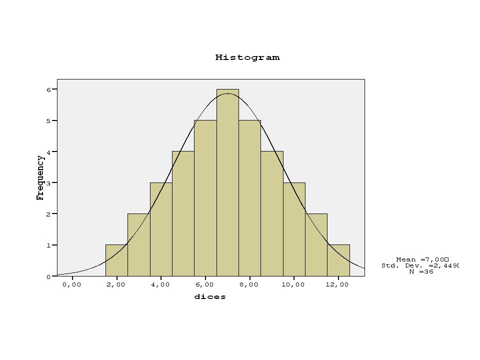
7. Probability Distribution Now, to see the distributions of the possible score, let’s compute the possibilities of each scores ranging between 2 – 12. Let’s relook at the table 1-11-21-31-41-51-6 2-12-22-32-42-52-6 3-13-23-33-43-53-6 4-14-24-34-44-54-6 5-15-25-35-45-55-6 6-16-26-36-46-56-6

8. Probability Distribution ScorefCum. fProp.cum prop. 121 360,0281 112 350,0560,972 103 330,0830,917 94 300,1110,833 85 260,1390,722 76 210,1670,583 65 150,1390,417 54 100,1110,278 43 60,0830,167 32 30,0560,083 21 10,028

9. Probability Distribution Now, let’s look at the shape of distribution.

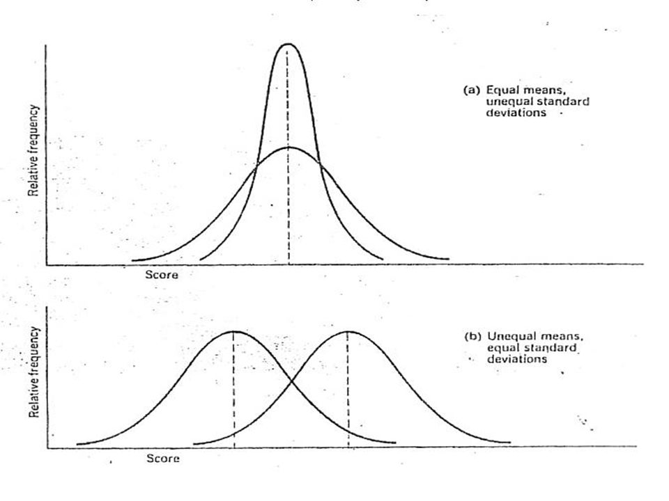
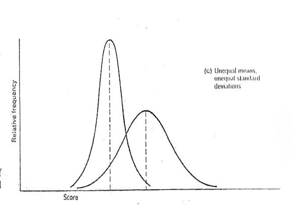
11. Basic Characteristics of Normal Curve There are different kinds of normal curves. Their means and standard deviations differ from each other. But, the matter of concern is their shape. Three possible conditions for normal curves are

14. Basic Characteristics of Normal Curve As you can see, the main similarity of the different normal curves is their symmetrical shape. – That is, the left half of the normal distribution is a mirror image of the right half They are unimodal distributions, with the mode at the center Mode, median and mean have the same value. Their tails never touches to the x axis. So, we describe the area under the curve as proportion. That is, the total area under the curve is equal to 1

15. Basic Characteristics of Normal Curve The equation of normal curve is:

16. Basic Characteristics of Normal Curve As you can see, the value of Y is determined by N, sd, mean. So, different distributions with different N, sd and mean have different normal distributions. Basically, N= the area under the curve Mean= location of the center of the curve SD= rapidity with which the curve approaches to x axis.

17. Basic Characteristics of Normal Curve As you can remember, to standardize different distributions, we use z scores. The mean and sd of z scores is 0 and 1, respectively. So, if we reorganize the formula for z, it becomes

18. Basic Characteristics of Normal Curve As you can see, last formula indicates that z score determines the area in the normal curve. So, using the standardized z scores, we can compute areas in the normal curve In book, you can see these areas in Table A, pp. 552

19. Area Under the Normal Curve In Table A, – z scores, – the area between z scores and mean, – and the area above z scores are presented. Note 1: the areas are bigger when z score is close to zero (the mean) Note 2: the sum of the two areas (the area between z scores and mean, AND the area above z scores) is.50. Because, this area represents the half of the distribution Note 3: All z scores in the distribution are positive, since the possitive area are the mirror image of negative area

20. Area Under the Normal Curve Using this table, we can calculate – The area above a certain score How many students (what proportion of scores) got (was) higher than 70 in the final prep. exam – The area under a certain score How many students got lower than 35 points in the final prep. exam – The area two known scores How many students got a score btw. 35 and 70 points in the final prep. exam

21. Area Under the Normal Curve The area above a certain score The mean of the prep. Final exm = 60 The SD is 10 2500 students took the final exam