Download presentation
Presentation is loading. Please wait.

1
Precise Digital Leveling
Section 4 Geodesy and Corrections for Leveling Precision Digital Leveling is a 1, 2, or 3 day seminar detailing the intricacies of geodetic leveling procedures developed by the National Geodetic Survey with emphasis on precise digital/bar-code levels and support equipment and how geodetic leveling is an integral part of Height Modernization. The seminar provides an overview of the geodetic leveling process including discussion of corrections applied to leveling, the FGCS specifications and procedures for electronic digital/bar-code leveling systems, required equipment, project reconnaissance, bench mark requirements and monumentation, field data collection, review, reduction, and “blue book” preparation for inclusion into the NGS National Spatial Reference System.

2
Leveled Height Differences
B Topography A C Leveling is a very “simple” survey practice - determining elevation differences through use of conventional leveling procedures – through backsight minus foresight measurements between points A to B and B to C. Differential leveling surveys, being a “piecewise” metric measurement technique, accumulate local height differences (dh). But, being a piecewise metric measurement system, we must also be aware and account for factors affecting our understanding and use of height interpretations. Traditionally, orthometric heights can be considered as a distance (elevation difference) above a reference surface or datum.
. But, being a piecewise metric measurement system, we must also be aware and account for factors affecting our understanding and use of height interpretations. Traditionally, orthometric heights can be considered as a distance (elevation difference) above a reference surface or datum.")
3
GRACE Gravity Model 01 - Released July 2003
To fully appreciate the reasoning for many of strict requirements for geodetic leveling we must begin with understanding what are orthometric heights. A realistic “view” of our very irregular shaped Earth as depicted in this gravity model determined from space borne gravity measurements by GRACE, gravity recovery and climate experiment. Every time we set up and plumb our level equipment we are then determining our horizon through the optics of the instrument perpendicular to the attraction of gravity at that point. Now, envision about 26 setups per mile and hundreds and thousands of setups over distances covering a County, each perpendicular to the attraction at that point on our irregular shaped, curved Earth and you can begin to get the feeling that leveling must be much more than a “simple” routine of backsights minus foresights. Image credit: University of Texas Center for Space Research and NASA

4
Geopotential The Geoid Surfaces Ellipsoid Surface Gravity Vector
Looking at a side view of the irregular shaped Earth and the relationships between surfaces of equal potential (equipotential or geopotential surfaces), perpendicular to the attraction of gravity at that point. Note these geopotential surfaces are not geometrically parallel due to the variations in the earth’s irregular gravity field. Also, the geopotential surfaces converge (become closer together) at the poles due in large part to Earth’s rotation. As you run levels across theses surfaces the equipment is plumbed per the attraction of gravity at that point. Our assumption is that our horizontal field of view can be corrected for a nice consistent Earth curvature when in fact a correction for conditions affecting us at a particular point must be accounted for. Running levels north and south require more correction for the convergence of the geopotential surfaces than when running levels east and west. The red oval illustrates the reference ellipsoid for our space based coordinate system and, though a close approximation of the size and shape of the Earth, is an entire, unrelated reference surface when determining GPS-derived ellipsoid heights. Gravity Vector The relationships between the ellipsoid surface (solid red), various geopotential surfaces (dashed blue), and the geoid (solid blue). The geoid exists approximately at mean sea level (MSL). Not shown is the actual surface of the earth, which coincides with MSL but is generally above the geoid.
, perpendicular to the attraction of gravity at that point. Note these geopotential surfaces are not geometrically parallel due to the variations in the earth’s irregular gravity field. Also, the geopotential surfaces converge (become closer together) at the poles due in large part to Earth’s rotation. As you run levels across theses surfaces the equipment is plumbed per the attraction of gravity at that point. Our assumption is that our horizontal field of view can be corrected for a nice consistent Earth curvature when in fact a correction for conditions affecting us at a particular point must be accounted for. Running levels north and south require more correction for the convergence of the geopotential surfaces than when running levels east and west. The red oval illustrates the reference ellipsoid for our space based coordinate system and, though a close approximation of the size and shape of the Earth, is an entire, unrelated reference surface when determining GPS-derived ellipsoid heights. Gravity Vector. The relationships between the ellipsoid surface (solid red), various geopotential surfaces (dashed blue), and the geoid (solid blue). The geoid exists approximately at mean sea level (MSL). Not shown is the actual surface of the earth, which coincides with MSL but is generally above the geoid.")
5
Level Surfaces and Orthometric Heights
Earth’s Surface WP Level Surfaces P Plumb Line Mean Sea Level “Geoid” WO PO Level surfaces - imagine earth standing still - ocean standing still; no effects such as currents, tides, winds; except for slight undulations created by gravity effects = level surface. Geoid is this level surface relating to today’s mean sea level surface - this does not truly coincide with mean sea level because of the non-averaging effects of currents, tides, water temperatures, salinity, weather, solar/lunar cycle, etc. The geoid is a best fit mean sea level surface. Equipotential surfaces - add or subtract water and level surface changes parallel to previous surface = infinite number of possible level surfaces. Each equipotential surface has one distinct potential quantity along its surface. Point on earth’s surface is the level surface parallel to the geoid achieved by adding or subtracting potential. Lines don’t appear parallel; they are based on the gravity field and are affected by mass pluses and minuses. Geopotential number is the numerical difference between two different equipotential surfaces. W = potential along a level surface. CP = geopotential number at a point. Plumb line (over exaggerated in drawing) - is a curved distance due to effects of direction of gravity- known as deflection of the vertical. Orthometric height is exactly the distance along this curved plumb line between the geoid and point on the earth’s surface. We can make close approximations but to be exact we would need to measure gravity along this line requiring a bored hole which is impractical. Level Surface = Equipotential Surface (W) Ocean Geopotential Number (CP) = WP -WO H (Orthometric Height) = Distance along plumb line (PO to P) Area of High Density Rock Area of Low Density Rock
 - is a curved distance due to effects of direction of gravity- known as deflection of the vertical. Orthometric height is exactly the distance along this curved plumb line between the geoid and point on the earth’s surface. We can make close approximations but to be exact we would need to measure gravity along this line requiring a bored hole which is impractical. Level Surface = Equipotential Surface (W) Ocean. Geopotential Number (CP) = WP -WO. H (Orthometric Height) = Distance along plumb line (PO to P) Area of High Density Rock. Area of Low Density Rock.")
6
Bench marks of NAVD 88 constitute the official national vertical datum for mapping and charting, and provide a vertical reference for the national infrastructure. Thus, surveyors frequently use these bench marks for reference points and to check their measurements. Leveled height differences (dh) do not strictly correspond to orthometric height differences (dH), because the nonparallelism of level surfaces is not reflected in the leveling measurements collected in the field (see figure); e.g., ∑dh (dh1+dh2+dh3) ≠ ∑dH (dH1+dH2+dH3) between bench marks A and B, where ∑dH = HB – HA. In contrast to leveled heights, adjusted NAVD 88 heights published by the National Geodetic Survey (NGS) are defined in the same Helmert orthometric vertical system as the orthometric heights obtained through the Global Positioning System (GPS) measurements and the proper geoid height value (apart from occasional small system shifts), such as the values provided by GEOID99.
 do not strictly correspond to orthometric height differences (dH), because the nonparallelism of level surfaces is not reflected in the leveling measurements collected in the field (see figure); e.g., ∑dh (dh1+dh2+dh3) ≠ ∑dH (dH1+dH2+dH3) between bench marks A and B, where ∑dH = HB – HA. In contrast to leveled heights, adjusted NAVD 88 heights published by the National Geodetic Survey (NGS) are defined in the same Helmert orthometric vertical system as the orthometric heights obtained through the Global Positioning System (GPS) measurements and the proper geoid height value (apart from occasional small system shifts), such as the values provided by GEOID99..")
7
Vertical Datum Relationships
3-D Datums WGS 84, NAD 83 (86) NAVD 88, NGVD 29 There are many ways to describe heights. Here are illustrated different “elevations” for the exact same point dependent on the measurement type and reference datum. Orthometric Datums Tidal Datums MHHW,MHW, MTL, DTL, MLW, MLLW
 NAVD 88, NGVD 29. There are many ways to describe heights. Here are illustrated different elevations for the exact same point dependent on the measurement type and reference datum. Orthometric Datums. Tidal Datums. MHHW,MHW, MTL, DTL, MLW, MLLW.")
8
Corrections Applied to NGS’ Leveling Observations
Source Documents: Balaz, Emery I., Young, Gary M.; NOAA Technical Memorandum NOS NGS 34; “CORRECTIONS APPLIED BY THE NATIONAL GEODETIC SURVEY TO PRECISE LEVELING OBSERVATIONS”; June 1982: FGCSVERT (ver /27/2004) The intent of this presentation is NOT to go into a discussion of how the following equations were derived, but rather, to familiarize the field observer about the variables which must be observed correctly in order to reduce leveling observations in conformance with NAVD88 conventions. The following corrections, and there are some either/or options, are used to reduce the rod readings to the geopotential numbers input to NGS’ geodetic leveling adjustment program: ASTA, and are the same corrections applied to the observations used to compute the NAVD88. Typeface coloring conventions: Black was used for the general points, Red was used to distinguish variables that the observers were directly involved in collecting.
 The intent of this presentation is NOT to go into a discussion of how the following equations were derived, but rather, to familiarize the field observer about the variables which must be observed correctly in order to reduce leveling observations in conformance with NAVD88 conventions. The following corrections, and there are some either/or options, are used to reduce the rod readings to the geopotential numbers input to NGS’ geodetic leveling adjustment program: ASTA, and are the same corrections applied to the observations used to compute the NAVD88. Typeface coloring conventions: Black was used for the general points, Red was used to distinguish variables that the observers were directly involved in collecting.")
9
Curvature Error, C, Where the Line of Sight
Is not Parallel to an Equipotential Surface Cancels if SB = SF Direction of Gravity SF SB CB CF Horizontal Line of Sight Equipotential Surface Our assumption is that the line of sight is perfectly horizontal, perpendicular to the attraction of gravity and that we work on a “flat” surface. We in fact live and work on a curved surface that is irregular due to the variable gravity influences in our world. The effects of curvature cancel if you maintain a close imbalance in your setups. FGCS Specifications and Procedures to Incorporate Electronic Digital/Bar-Code Leveling Systems: Difference of forward and backward sight lengths never to exceed: 5 m per setup and 10 m per section for 1st and 2nd Order leveling.

10
Shorten setup distances – instrument to rod
Rod A Rod B Shimmer Refraction is most notable when the line of sight passes through air of fluctuating density, as when “heat waves” are observed. The graduations on the scales appear to move up and down rapidly. This phenomenon, called shimmer, makes it difficult to intercept the scales precisely, thus increasing the magnitude of pointing error. It can be reduced by shortening the sighting distances or, in some cases, raising the height of the line of sight. Balanced setups tend to cancel some effects of shimmer if conditions are the same in both the backsight and foresight observations. Important Note: Observe over similar surfaces in backsight and foresight observations. This becomes very apparent when crossing roadways as the backsight may be along the road shoulder but the foresight across an asphalt highway would be over a dissimilar surface. Cross the highway at nearly a right angle which requires a setup with reduced distances backsight and foresight to help minimize the effects observing over dissimilar surfaces. Shorten setup distances – instrument to rod Balance setups – minimize differences Observe over similar surfaces

11
Crossing a Highway Avoid if Possible Minimize Dissimilar Backsight -
Foresight Observing Conditions Important Note and Example: Observe over similar surfaces in backsight and foresight observations. This becomes very apparent when crossing roadways as the backsight may be along the road shoulder but the foresight across an asphalt highway would be over a dissimilar surface. Cross the highway at nearly a right angle which requires a setup with reduced distances backsight and foresight to help minimize the effects observing over dissimilar surfaces.

12
F1cos P2 B2cos P2 B1cos P1 Rod 1 Rod 2 F2cos P1 To observe accurate heights above the points on which the leveling rods rest, precise relationships must be maintained between the rods and the equipotential surface, and between the rods and the scales mounted on them. This is ensured by plumbing, or aligning the rods with the direction of gravity, a task which is analogous to leveling the instrument. If they are not aligned, an error is introduced into each observation. Although the error may be small, it accumulates systematically with change of elevation, especially on steep slopes where observations are made alternately low and high on scale. It can be limited only by plumbing the scales properly. Systematic effect of plumbing error (and scale errors) is small on flat terrain, since B1 ≈ F2 and F1 ≈ B2
 is small on flat terrain, since B1 ≈ F2 and F1 ≈ B2.")
13
Rod 1 Rod 2 Rod 1 F2cos P1 B2cos P2 F1cos P2 B1cos P1 Again, it is important to ensure the rods are plumb at every setup. If they are not aligned, an error is introduced into each observation. Although the error may be small, it accumulates systematically with change of elevation, especially on steep slopes where observations are made alternately low and high on scale. It can be limited only by plumbing the scales properly. Systematic effect of plumbing error (and scale errors) accumulates on sloping terrain, since B1 ≠ F2 and F1 ≠ B2
 accumulates on sloping terrain, since B1 ≠ F2 and F1 ≠ B2.")
15
Checking rod plumb: During a setup each leveling rod must be plumb, in other words, vertically aligned with the direction of gravity .. Achieve this by centering the bubble in the vial of the circular level attached to the rod housing. To center the bubble precisely, use a mirror or reflecting prism mounted on the rod to observe the level from as nearly overhead as possible, not from the side. Each day, while leveling, the observer should check the plumbing of each rod by comparing the alignment of each rod to the vertical line in the reticle of the leveling instrument. Check the rod while it faces the instrument; then, after the rodman turns the rod 90' (at a right angle to the instrument), check it again. This procedure quickly reveals gross errors in the plumbing of the rod. If the circular level is not properly adjusted, centering the bubble does not ensure that the rod is plumb. Check the level by one of the following methods at least once a week and immediately after any shock to the rod. Include a note in each weekly report, stating the time and date that the check was performed, and explaining the adjustments required. If the level cannot be adjusted within tolerance, the rod housing may be warped or the level may be defective. In this case, check the housing by stretching a string from one end of the rod to the other and looking for bends or twists, If the rod has such defects, replace it immediately. If not, replace the circular level. NOAA Manual NOS NGS 3, Geodetic Leveling; 3.4 Leveling Rods; Use and Maintenance
, check it again. This procedure quickly. reveals gross errors in the plumbing of the rod. If the circular level is not properly adjusted, centering the bubble does not ensure that the rod is plumb. Check the level by one of the following methods at least once a week and immediately after any shock to the rod. Include a note in each weekly report, stating the time and date that the check was performed, and explaining the adjustments required. If the level cannot be adjusted within tolerance, the rod housing may be warped or the level may be defective. In this case, check the housing by stretching a string from one end of the rod to the other and looking for bends or twists, If the rod has such defects, replace it immediately. If not, replace the circular level. NOAA Manual NOS NGS 3, Geodetic Leveling; 3.4 Leveling Rods; Use and Maintenance.")
16
Rod Scale Correction Cr = De
D = observed Δelevation for the section in meters e = average length excess of the rod pair in mm/m Length excess is determined in rod calibration process The length of the Invar strip of a leveling rod used in precise leveling should be traceable to the National length standard. While they should be calibrated before and after each project or at least once a year, this has never been deemed practical except when the client has “deep pockets” and has told NGS they wanted the “best” inferring 1st Order, Class I leveling. In practice, the rods are calibrated before one uses them for a precise leveling project, and then, possibly if they’ve been in storage for a long while, so when “dusted off” still look new and/or the ownership of the rods has changed and the new owner is uncertain about the quality of the original certification. While the rods should be recalibrated after they are damaged, most users would rather buy and calibrate new rods than repair and recalibrate a damaged rod set. Also, handling quickly wears painted surfaces off the rods, thus they often get retired before the true end of their useful life. You get two useful values out of a rod calibration; one is related to the thermal index of refraction of the Invar strip, and the other is related to the distance between the bottom of the rod (the part that contacts the monument) and the “zero point” on each strip. Now, most geodetic rods really don’t display “ ”. More likely they display a different range of numbers that were chosen by the manufacturer to catch blunders because certain combinations of differences as measured by the backsight followed by the foresight would be impossible if both rods started with “zero.” This thinking then leads to the procedural technique that says you always quit the section on a Bench Mark with the same rod as you used when you started the section on another Bench Mark. This correction deals with the differences between the bottom of the rod and the “zero point.” Now, since 1980, NGS would like the calibration to include more than one “zero point” so we can do a least squares determination of all the check points which are related to the foot of the rod. When the National Bureau of Standards was doing them we got them every 10cm along the rod. More recently, non NIST labs doing calibrations have only been producing one index value per meter along the rod. NGS accepts these calibrations but wishes the labs would produce more fiducial point comparisons. Source Documents: Balaz, Emery I., Young, Gary M.; NOAA Technical Memorandum NOS NGS 34; “CORRECTIONS APPLIED BY THE NATIONAL GEODETIC SURVEY TO PRECISE LEVELING OBSERVATIONS”; June 1982: FGCSVERT (ver /27/2004)
 and the zero point on each strip. Now, most geodetic rods really don’t display More likely they display a different range of numbers that were chosen by the manufacturer to catch blunders because certain combinations of differences as measured by the backsight followed by the foresight would be impossible if both rods started with zero. This thinking then leads to the procedural technique that says you always quit the section on a Bench Mark with the same rod as you used when you started the section on another Bench Mark. This correction deals with the differences between the bottom of the rod and the zero point. Now, since 1980, NGS would like the calibration to include more than one zero point so we can do a least squares determination of all the check points which are related to the foot of the rod. When the National Bureau of Standards was doing them we got them every 10cm along the rod. More recently, non NIST labs doing calibrations have only been producing one index value per meter along the rod. NGS accepts these calibrations but wishes the labs would produce more fiducial point comparisons. Source Documents: Balaz, Emery I., Young, Gary M.; NOAA Technical Memorandum NOS NGS 34; CORRECTIONS APPLIED BY THE NATIONAL GEODETIC SURVEY TO PRECISE LEVELING OBSERVATIONS ; June 1982: FGCSVERT (ver /27/2004)")
17
Rod Calibration – Invar to Bottom Reference Plate
Rod scale is the distance between the bottom of the rod (the part that contacts the monument) and the “zero point” on each Invar strip.
 and the zero point on each Invar strip.")
18
Calibration Report SLAC Metrology Laboratory
An example “paper” rod calibration report and a picture of the Stanford Linear Accelerator Center (SLAC) rod calibration setup in a climate controlled laboratory. The rods used for geodetic leveling must be calibrated routinely by a reputable laboratory against a standard that has been compared to the National Standard of Length. A complete set of calibration data should be obtained for each rod before the rod is first used, every 5 years during its use, and just before the rod or scale is retired. The data should include the index error, length excess, and coefficient of thermal expansion. In addition, during each year of use, at least one calibration should be made to determine the index error and length excess. If a rod is dropped, or otherwise handled in a way that may have damaged it, it should not be used again until it has been recalibrated. Each calibration consists of the precise measurement of at least four overlapping intervals on the scale (usually between the base plate and the bisected graduations at 0.2, 1.0, 2.0, and 3.0 m). The measurements, with respect to the National Standard of Length, should be accurate to ± 0.05 mm. From one calibration, a value for the index error and a factor for the length excess can be computed. The differences between the calibrated and assigned lengths of the graduations are plotted versus the assigned lengths. The intercept of the plotted line with the axis of the differences is the index correction which is equal and opposite in sign to the index error. The slope of the line is the length excess. To obtain a complete set of calibration data, at least four calibrations must be made, each at a different temperature between 15° and 35°C. The variations in graduation values, due to changes in temperature, are described by the coefficient of thermal expansion, computed from these data. NOAA Manual NOS NGS 3, Geodetic Leveling; 3.4 Leveling Rods; Calibration SLAC Metrology Laboratory
 rod calibration setup in a climate controlled laboratory. The rods used for geodetic leveling must be calibrated routinely by a reputable laboratory against a standard that has been compared to the National Standard of Length. A complete set of calibration data should be obtained for each rod before the rod is first used, every 5 years during its use, and just before the rod or scale is retired. The data should include the index error, length excess, and coefficient of thermal expansion. In addition, during each year of use, at least one calibration should be made to determine the index error and length excess. If a rod is dropped, or otherwise handled in a way that may have damaged it, it should not be used again until it has been recalibrated. Each calibration consists of the precise measurement of at least four overlapping intervals on the scale (usually between the base plate and the bisected graduations at 0.2, 1.0, 2.0, and 3.0 m). The measurements, with respect to the National Standard of Length, should be accurate to ± 0.05 mm. From one calibration, a value for the index error and a factor for the length excess can be computed. The differences between the calibrated and assigned lengths of the graduations are plotted versus the assigned lengths. The intercept of the plotted line with the axis of the differences is the index correction which is equal and opposite in sign to the index error. The slope of the line is the length excess. To obtain a complete set of calibration data, at least four calibrations must be made, each at a different temperature between 15° and 35°C. The variations in graduation values, due to changes in temperature, are described by the coefficient of thermal expansion, computed from these data. NOAA Manual NOS NGS 3, Geodetic Leveling; 3.4 Leveling Rods; Calibration. SLAC Metrology Laboratory.")
19
Laval University (ULAVAL)
An example “paper” rod calibration report from the Laval University in Quebec, Canada.

20
Technical University in Munich (TUM)
An example “paper” rod calibration report from the Technical University in Munich, Germany (TUM).
.")
21
Stanford Linear Accelerator Center (SLAC)
An example “paper” rod calibration report from the Stanford Linear Accelerator Center (SLAC). Stanford Linear Accelerator Center Metrology Department 2575 Sand Hill Road, Menlo Park, CA 94025 Tel.: (650) , Fax: (650)
. Stanford Linear Accelerator Center. Metrology Department Sand Hill Road, Menlo Park, CA Tel.: (650) , Fax: (650)")
22
Stanford Linear Accelerator Center (SLAC) Additional Notes
3 Notes and Recommendations; 3.1 Visual inspection of the rods: Figure 1: Footplate of both rods. Both rods show wear at the center of the footplate, indicating that they have been set up in the center. The correct spot to set up the rods is not the center of the footplate. The rods should be set up in line with the scale itself, indicated with a green dot in the picture above. This mitigates errors if the rod is not set up perfectly straight. Figure 2: Strap in front of code. The DNA03 uses a ~1 deg section of the code visible at its CCD array. No section of the code should be covered. In the image above, the modification of the strap covers a small portion of it. System Calibration Report; GPCL3 Rod (SN: 26923)– GPCL3 Rod (SN: 26924); Leica DNA03 (SN: )
– GPCL3 Rod (SN: 26924); Leica DNA03 (SN: )")
23
Critical Distances: It is already well known in the metrology community that digital levels give inaccurate results at certain distances. Therefore the expansion of these distances have to be evaluated to avoid them during the field measurements. As an example, measurements at and around a critical distance of the DNA03 are shown below. Stanford Linear Accelerator Center (SLAC) rod calibration report including information on critical distances. Precision in height measurements is reduced at these critical distances. It is already well known in the metrology community that digital levels give inaccurate results at certain distances. Therefore the expansion of these distances have to be evaluated to avoid them during the field measurements. As an example, measurements at and around a critical distance of the DNA03 are shown. Some of the manufacturers have built these “critical” distances into their digital level firmware and a warning is indicated prohibiting readings when these critical distances are encountered in the field.
 rod calibration report including information on critical distances. Precision in height measurements is reduced at these critical distances. It is already well known in the metrology community that digital levels give inaccurate results at certain distances. Therefore the expansion of these distances have to be evaluated to avoid them during the field measurements. As an example, measurements at and around a critical distance of the DNA03 are shown. Some of the manufacturers have built these critical distances into their digital level firmware and a warning is indicated prohibiting readings when these critical distances are encountered in the field.")
24
Hence Rule – Keep all three crosshairs on Invar!
Stanford Linear Accelerator Center (SLAC) rod calibration report including information on readings near the ends of staff. Precision in height measurements is reduced when observing near the ends of the rods. For determination of the height reading, a certain area of the code on the leveling rod is used by the level. If only parts of this area are visible, as is the case at the end sections of the staff, inaccurate measurements are the consequence. Some of the manufacturers of digital levels have built user input limitations for high or low staff readings into their leveling routine and a warning is indicated prohibiting readings when exceeding these limitations are encountered in the field. Hence Rule – Keep all three crosshairs on Invar!
 rod calibration report including information on readings near the ends of staff. Precision in height measurements is reduced when observing near the ends of the rods. For determination of the height reading, a certain area of the code on the leveling rod is used by the level. If only parts of this area are visible, as is the case at the end sections of the staff, inaccurate measurements are the consequence. Some of the manufacturers of digital levels have built user input limitations for high or low staff readings into their leveling routine and a warning is indicated prohibiting readings when exceeding these limitations are encountered in the field. Hence Rule – Keep all three crosshairs on Invar!")
25
Keep all three crosshairs on Invar!
As a procedural routine, keep all three crosshairs on the Invar of the rod to force reading below the top (or bottom) 10 cm where the precision in height measurements is reduced when observing near the ends of the rods. For determination of the height reading, a certain area of the code on the leveling rod is used by the level. If only parts of this area are visible, as is the case at the end sections of the staff, inaccurate measurements are the consequence. Some of the manufacturers of digital levels have built user input limitations for high or low staff readings into their leveling routine and a warning is indicated prohibiting readings when exceeding these limitations are encountered in the field. Keep all three crosshairs on Invar!
 10 cm where the precision in height measurements is reduced when observing near the ends of the rods. For determination of the height reading, a certain area of the code on the leveling rod is used by the level. If only parts of this area are visible, as is the case at the end sections of the staff, inaccurate measurements are the consequence. Some of the manufacturers of digital levels have built user input limitations for high or low staff readings into their leveling routine and a warning is indicated prohibiting readings when exceeding these limitations are encountered in the field. Keep all three crosshairs on Invar!")
26
Maintain Line of Sight 0.5 m Above Ground
Rod Must be ≥ 0.5 m 0.5 m Leveling; a “simple” form of surveying - transferring elevation differences through a series of backsight minus foresight measurements. Geodetic Glossary: Leveling - Leveling between two points relatively close to each other (within 2-3 meters vertically, and less than 100 meters horizontally) is done by holding a graduated leveling rod vertically at each point and reading, with a horizontal telescope placed midway between the two points, the place where each rod intersects the horizontal plane established by the telescope's line of sight. The difference in readings is, approximately, the difference in elevation. If the points are farther apart than the distances mentioned above, measurements are made at shorter distance intervals and the total difference in elevation is taken as the sum of the resulting smaller measured differences. The elevation of a point is determined by proceeding as above, starting at a point that is either on the reference surface or at a previously determined elevation. The desired elevation is called the orthometric elevation; quantities approximating the orthometric elevation and derived from the measurements by applying various kinds of corrections are given special names such as Helmert height, Niethammer elevation, and the like. This is a single setup of leveling. A leveling instrument placed halfway between two leveling rods with precise graduations. The elevation at the beginning point, supporting rod 1, is transferred to the instrument through a measurement at the back rod (backsight) along with a distance (stadia distance) from the rod to the instrument. The elevation is then transferred from the instrument through a measurement at the front rod (foresight) along with a distance (stadia distance) from the instrument to the rod. The imbalance between the backsight and foresight distances must be kept to a minimum. The elevation has then been transferred to the point supporting rod 2.
 is done by holding a graduated leveling rod vertically at each point and reading, with a horizontal telescope placed midway between the two points, the place where each rod intersects the horizontal plane established by the telescope s line of sight. The difference in readings is, approximately, the difference in elevation. If the points are farther apart than the distances mentioned above, measurements are made at shorter distance intervals and the total difference in elevation is taken as the sum of the resulting smaller measured differences. The elevation of a point is determined by proceeding as above, starting at a point that is either on the reference surface or at a previously determined elevation. The desired elevation is called the orthometric elevation; quantities approximating the orthometric elevation and derived from the measurements by applying various kinds of corrections are given special names such as Helmert height, Niethammer elevation, and the like. This is a single setup of leveling. A leveling instrument placed halfway between two leveling rods with precise graduations. The elevation at the beginning point, supporting rod 1, is transferred to the instrument through a measurement at the back rod (backsight) along with a distance (stadia distance) from the rod to the instrument. The elevation is then transferred from the instrument through a measurement at the front rod (foresight) along with a distance (stadia distance) from the instrument to the rod. The imbalance between the backsight and foresight distances must be kept to a minimum. The elevation has then been transferred to the point supporting rod 2.")
27
RI-LOAD Documentation
Detailed level instrument and rod calibration data are stored in the National Geodetic Survey’s (NGS) integrated data base (NGSIDB) to apply corrections by the processing programs to the leveling data contained in the leveling observations file (*.hgz) in an attempt to remove systematic errors from the observations. This generates a “phase 1” file (*.ph1) which theoretically has only random errors remaining. The phase 1 file (*.ph1) can be used as input for the least-squares adjustment process which is applicable only if errors are random in nature. The information about the level instrument and rod is added into the NGSIDB through coded load-files which are created on the basis of an internal NGS document, RILOAD.wpd. Additional descriptive information can be found in the Input Formats and Specifications of the National Geodetic Survey Data Base, known as the “Blue Book” and available from the NGS Web site at: The fields in the data input record are comma separated. The specified widths for each field are the maximum spaces allowable. Tabs and other special characters are not allowed nor should fields be enclosed in quotes. A field may have any number of leading and trailing blanks as the RILOAD program will remove leading or trailing blanks from each field before processing. Embedded blanks in strings are considered to be part of the string. All data input records are case insensitive. Wildcards are NOT allowed in any data input commands.
 integrated data base (NGSIDB) to apply corrections by the processing programs to the leveling data contained in the leveling observations file (*.hgz) in an attempt to remove systematic errors from the observations. This generates a phase 1 file (*.ph1) which theoretically has only random errors remaining. The phase 1 file (*.ph1) can be used as input for the least-squares adjustment process which is applicable only if errors are random in nature. The information about the level instrument and rod is added into the NGSIDB through coded load-files which are created on the basis of an internal NGS document, RILOAD.wpd. Additional descriptive information can be found in the Input Formats and Specifications of the National Geodetic Survey Data Base, known as the Blue Book and available from the NGS Web site at: The fields in the data input record are comma separated. The specified widths for each field are the maximum spaces allowable. Tabs and other special characters are not allowed nor should fields be enclosed in quotes. A field may have any number of leading and trailing blanks as the RILOAD program will remove leading or trailing blanks from each field before processing. Embedded blanks in strings are considered to be part of the string. All data input records are case insensitive. Wildcards are NOT allowed in any data input commands.")
28
Leveling instruments are passive measurement systems that use ambient light to read the rods. In tunnels, we use flashlights to illuminate the rods and allow measurements. Therefore tests with our instruments have to be carried out to find out if the inhomogeneous illumination of flashlights has an effect or not. By taking more then 100 measurements at a sighting distance of 3 m, illuminating the staff with a flashlight (Black & Decker Snake Light) in front of the rod and up to an angle of about 45°, either no measurements were taken or the measurements were correct. But taking measurements with the illumination at a very steep angle (see Figure 5) deviations of up to 0.1 mm could be invoked. This can be explained by a shadowing effect of the code elements. During the manufacturing process the whole scale is first covered with a black layer and then with a yellow layer. The top yellow layer is removed with a high energy laser to make the black color visible. Due to this process the code elements have a certain thickness of a few micrometers, Fischer and Fischer (1999).
 in front of the rod and up to an angle of about 45°, either no measurements were taken or the measurements were correct. But taking measurements with the illumination at a very steep angle (see Figure 5) deviations of up to 0.1 mm could be invoked. This can be explained by a shadowing effect of the code elements. During the manufacturing process the whole scale is first covered with a black layer and then with a yellow layer. The top yellow layer is removed with a high energy laser to make the black color visible. Due to this process the code elements have a certain thickness of a few micrometers, Fischer and Fischer (1999).")
29
Rod Temperature Correction
Ct = ( tm – ts ) D · CE tm = mean observed temperature of Invar strip ts = standardization temperature of Invar strip D = observed Δelevation between the bench marks CE = mean coefficient of thermal expansion This is the second correction that comes out of information determined during the rod calibration procedure. The ambient air temperature should be measured and recorded to the nearest degree F or 0.5 degree C at the beginning of the section and the end of the section; the appropriate units (C or F) noted and/or recorded. Source Documents: Balaz, Emery I., Young, Gary M.; NOAA Technical Memorandum NOS NGS 34; “CORRECTIONS APPLIED BY THE NATIONAL GEODETIC SURVEY TO PRECISE LEVELING OBSERVATIONS”; June 1982: FGCSVERT (ver /27/2004)
 D · CE. tm = mean observed temperature of Invar strip. ts = standardization temperature of Invar strip. D = observed Δelevation between the bench marks. CE = mean coefficient of thermal expansion. This is the second correction that comes out of information determined during the rod calibration procedure. The ambient air temperature should be measured and recorded to the nearest degree F or 0.5 degree C at the beginning of the section and the end of the section; the appropriate units (C or F) noted and/or recorded. Source Documents: Balaz, Emery I., Young, Gary M.; NOAA Technical Memorandum NOS NGS 34; CORRECTIONS APPLIED BY THE NATIONAL GEODETIC SURVEY TO PRECISE LEVELING OBSERVATIONS ; June 1982: FGCSVERT (ver /27/2004)")
30
Refraction Correction (thermistors)
R = γ(S/50)2 δ · D S = distance (instrument to rod) in meters γ = 70 δ = observed temperature difference between probes at each setup D = Δelevation for the setup in units of half-cm This is required for all leveling of O/C equal to and greater than 2/1. 2/2 leveling may be done without observing the temperature gradient but it is preferred if probes and this method is used. The probes need to be compared at the start and end of every day and when one is “suspicious” of the observations. This is done by bringing the two probes to the same height and comparing the readings. The two probe temperature readings thus compared should not disagree by more than 0.2° C. If they do, then they should be adjusted so that they do. This is “pretty automatic” when the digital level is set up properly. Distance “S” is the stadia distance and the instrument reads and normally records it. The elevation difference, of course comes from the rod readings and the digital level Bluebooking program should take care of converting the elevation difference into units of half-cm. The observer just has to be careful about remembering to read the probes and enter the read values correctly into the appropriate variables via the keypad on the instrument. Some manufacturer’s may even allow a programmer to “filter” the readings to observer punches in to trap “fat fingering” blunders. Source Documents: Balaz, Emery I., Young, Gary M.; NOAA Technical Memorandum NOS NGS 34; “CORRECTIONS APPLIED BY THE NATIONAL GEODETIC SURVEY TO PRECISE LEVELING OBSERVATIONS”; June 1982: FGCSVERT (ver /27/2004).
2 δ · D. S = distance (instrument to rod) in meters. γ = 70. δ = observed temperature difference. between probes at each setup. D = Δelevation for the setup in units of half-cm. This is required for all leveling of O/C equal to and greater than 2/1. 2/2 leveling may be done without observing the temperature gradient but it is preferred if probes and this method is used. The probes need to be compared at the start and end of every day and when one is suspicious of the observations. This is done by bringing the two probes to the same height and comparing the readings. The two probe temperature readings thus compared should not disagree by more than 0.2° C. If they do, then they should be adjusted so that they do. This is pretty automatic when the digital level is set up properly. Distance S is the stadia distance and the instrument reads and normally records it. The elevation difference, of course comes from the rod readings and the digital level Bluebooking program should take care of converting the elevation difference into units of half-cm. The observer just has to be careful about remembering to read the probes and enter the read values correctly into the appropriate variables via the keypad on the instrument. Some manufacturer’s may even allow a programmer to filter the readings to observer punches in to trap fat fingering blunders. Source Documents: Balaz, Emery I., Young, Gary M.; NOAA Technical Memorandum NOS NGS 34; CORRECTIONS APPLIED BY THE NATIONAL GEODETIC SURVEY TO PRECISE LEVELING OBSERVATIONS ; June 1982: FGCSVERT (ver /27/2004).")
31
Refraction Error, r, Does Not Cancel on
Sloping Terrain Since rB ≠ rF, even if SB = SF Cool rF rB Refraction. Variations in atmospheric density cause the line of sight to refract or bend in the direction of increasing air density. These variations seem to be primarily a function of air temperature. Refraction is most noticeable when the line of sight passes through air of fluctuating density. As long as atmospheric conditions are similar along both the foresight and backsight, the error may be nearly eliminated by balancing setups. However, conditions are often not the same along both lines of sight. Air close to the ground changes in density more rapidly than air situated 1 m or more above ground. This can be visualized by imagining air layers, of equal density, conforming to the topography. On a slope, even if setups are exactly balanced, the conditions along the foresight differ from those along the backsight. Because the sight uphill passes through a greater change in air density, it is refracted more. Refraction error, then, accumulates with change in elevation. NOAA Manual NOS NGS 3, Geodetic Leveling; 3.1 Introduction; Sources of Error Warm SB SF

32
NGS Aspirated Temperature Probes
Example of the NGS manufactured, manually read and recorded, thermistor unit mounted on a rigid leg tripod. Leveling results may be corrected at least partially for refraction if atmospheric conditions are determined and recorded with the observations. Of the many mathematical models that attempt to predict refraction error, the most successful require that air-temperature differences be precisely measured during every setup. NOAA Manual NOS NGS 3, Geodetic Leveling; 3.1 Introduction; Sources of Error Measuring air-temperature difference: The best mathematical models for computing refraction corrections depend upon measuring at least one air temperature difference during every setup. Temperatures are measured at two different heights above the ground. The difference is computed by subtracting the temperature at the bottom from that at the top. It is usually negative during daylight hours when the Sun heats the ground, warming the lower air layers. It is positive when the air near the ground is cooler than that above it. Use aspirated thermometers, accurate to ± 0. l° C (± 0.2° F), to measure the temperature difference. A typical measuring system includes two thermistors, each shaded by a metal tube and aspirated by a small, battery powered fan. A digital display permits readings to be made from either thermistor. Air movement across the thermistors should be equal at all times. Check for air movement by placing your hand in front of each thermistor. NOAA Manual NOS NGS 3, Geodetic Leveling; 3.6 Atmospheric Conditions; Air Temperature, Sun, and Wind
, to measure the temperature difference. A typical measuring system includes two thermistors, each shaded by a metal tube and aspirated by a small, battery powered fan. A digital display permits readings to be made from either thermistor. Air movement across the thermistors should be equal at all times. Check for air movement by placing your hand in front of each thermistor. NOAA Manual NOS NGS 3, Geodetic Leveling; 3.6 Atmospheric Conditions; Air Temperature, Sun, and Wind.")
33
Rigid Leg Tripod With Thermister Equipment
Example of the NGS manufactured, manually read and recorded, thermistor unit mounted on a rigid leg tripod. Leveling results may be corrected at least partially for refraction if atmospheric conditions are determined and recorded with the observations. Of the many mathematical models that attempt to predict refraction error, the most successful require that air-temperature differences be precisely measured during every setup. NOAA Manual NOS NGS 3, Geodetic Leveling; 3.1 Introduction; Sources of Error Measuring air-temperature difference: The best mathematical models for computing refraction corrections depend upon measuring at least one air temperature difference during every setup. Temperatures are measured at two different heights above the ground. The difference is computed by subtracting the temperature at the bottom from that at the top. It is usually negative during daylight hours when the Sun heats the ground, warming the lower air layers. It is positive when the air near the ground is cooler than that above it. Use aspirated thermometers, accurate to ± 0. l° C (± 0.2° F), to measure the temperature difference. A typical measuring system includes two thermistors, each shaded by a metal tube and aspirated by a small, battery powered fan. A digital display permits readings to be made from either thermistor. Air movement across the thermistors should be equal at all times. Check for air movement by placing your hand in front of each thermistor. NOAA Manual NOS NGS 3, Geodetic Leveling; 3.6 Atmospheric Conditions; Air Temperature, Sun, and Wind
, to measure the temperature difference. A typical measuring system includes two thermistors, each shaded by a metal tube and aspirated by a small, battery powered fan. A digital display permits readings to be made from either thermistor. Air movement across the thermistors should be equal at all times. Check for air movement by placing your hand in front of each thermistor. NOAA Manual NOS NGS 3, Geodetic Leveling; 3.6 Atmospheric Conditions; Air Temperature, Sun, and Wind.")
34
Refraction Correction (predicted)
R = γ{S/[(2n)(50)}2 δ · d · W S = distance (instrument to rod) in meters γ = 70 n = number of setups δ = “predicted” temp. diff. d = Δelevation for the setup in units of half-cm W = weather factor based upon “sun code” where it equals 0.5 for totally overcast, 1.0 for 50% cloudy, 1.5 for 100% sunny Correction not used when thermistors are used! This reduction is used for Second-order Class II and lower leveling when information for computing the temperature gradient is not provided by the observer, and when, occasionally, reductions using the temperature values provided do “not work” for Second-Order Class I and higher-order leveling. Now in the case of Second-order Class I and higher, don’t expect this fallback procedure to be used for more than a couple of sections in the entire project! What is being said here is just because temperature gradients are being observed does NOT mean the observer can neglect observing “sun codes”. Now, the model that uses these sun codes is dependent upon the time of observation and the position of the section’s starting and ending Bench Marks. So be sure to record times of observation – and their time zones, and get the position correct in the associated description! Source Documents: Balaz, Emery I., Young, Gary M.; NOAA Technical Memorandum NOS NGS 34; “CORRECTIONS APPLIED BY THE NATIONAL GEODETIC SURVEY TO PRECISE LEVELING OBSERVATIONS”; June 1982: FGCSVERT (ver /27/2004).
(50)}2 δ · d · W. S = distance (instrument to rod) in meters. γ = 70. n = number of setups. δ = predicted temp. diff. d = Δelevation for the setup in units of half-cm. W = weather factor based upon sun code where it equals 0.5 for totally overcast, 1.0 for 50% cloudy, 1.5 for 100% sunny. Correction not used when thermistors are used! This reduction is used for Second-order Class II and lower leveling when information for computing the temperature gradient is not provided by the observer, and when, occasionally, reductions using the temperature values provided do not work for Second-Order Class I and higher-order leveling. Now in the case of Second-order Class I and higher, don’t expect this fallback procedure to be used for more than a couple of sections in the entire project! What is being said here is just because temperature gradients are being observed does NOT mean the observer can neglect observing sun codes . Now, the model that uses these sun codes is dependent upon the time of observation and the position of the section’s starting and ending Bench Marks. So be sure to record times of observation – and their time zones, and get the position correct in the associated description! Source Documents: Balaz, Emery I., Young, Gary M.; NOAA Technical Memorandum NOS NGS 34; CORRECTIONS APPLIED BY THE NATIONAL GEODETIC SURVEY TO PRECISE LEVELING OBSERVATIONS ; June 1982: FGCSVERT (ver /27/2004).")
35
U.S. NAVY TIME ZONE DESIGNATIONS
Time Zones U.S. NAVY TIME ZONE DESIGNATIONS STANDARD DAYLIGHT TIME TIME ZONE U.S.NAVY TIME TIME MERIDIAN DESCRIP’N DESIGNATION Atlantic AST Eastern EDT 60W Q (Quebec) Eastern EST Central CDT 75W R (Romeo) Central CST Mountain MDT 90W S (Sierra) Mountain MST Pacific PDT 105W T (Tango) Pacific PST Yukon YDT 120W U (Uniform) Yukon YST AK/HI HDT 135W V (Victor) AK/HI HST Bering BDT 150W W (Whiskey) Note the zone letter changes when you change from STANDARD time to DAYLIGHT time. Previous slides mentioned the importance recording the time zone correctly. The recorded date, time zone, and time must be accurate because observations are stored and sorted chronologically. Corrections for collimation error, refraction, tidal accelerations, and scale error are applied accordingly. Time zones should be coded according to the alphabetical system of the U.S. Navy. NOAA Manual NOS NGS 3, Geodetic Leveling; 3.8 Field Records; Recording Observations
 Eastern EST Central CDT 75W +5 R (Romeo) Central CST Mountain MDT 90W +6 S (Sierra) Mountain MST Pacific PDT 105W +7 T (Tango) Pacific PST Yukon YDT 120W +8 U (Uniform) Yukon YST AK/HI HDT 135W +9 V (Victor) AK/HI HST Bering BDT 150W +10 W (Whiskey) Note the zone letter changes when you change from STANDARD time to DAYLIGHT time. Previous slides mentioned the importance recording the time zone correctly. The recorded date, time zone, and time must be accurate because observations are stored and sorted chronologically. Corrections for collimation error, refraction, tidal accelerations, and scale error are applied. accordingly. Time zones should be coded according to the alphabetical system of the U.S. Navy. NOAA Manual NOS NGS 3, Geodetic Leveling; 3.8 Field Records; Recording Observations.")
36
Astronomic Correction
Ca = 0.7 · Ks s = section length K = tan εm cos(Am – α) + tan εs cos(As – α) where As = azimuth of the sun; Am = azimuth of the moon; α = azimuth of section (Δλ/Δθ of adjacent BMs) 0.7 because the earth is elastic The astronomic correction model uses the time of day as well as the position of the Bench Marks to compute the azimuths of the Sun and Moon, so once again, those positions in the description and those recorded times and zones are very important. Source Documents: Balaz, Emery I., Young, Gary M.; NOAA Technical Memorandum NOS NGS 34; “CORRECTIONS APPLIED BY THE NATIONAL GEODETIC SURVEY TO PRECISE LEVELING OBSERVATIONS”; June 1982: FGCSVERT (ver /27/2004).
 + tan εs cos(As – α) where As = azimuth of the sun; Am = azimuth of the moon; α = azimuth of section (Δλ/Δθ of adjacent BMs) 0.7 because the earth is elastic. The astronomic correction model uses the time of day as well as the position of the Bench Marks to compute the azimuths of the Sun and Moon, so once again, those positions in the description and those recorded times and zones are very important. Source Documents: Balaz, Emery I., Young, Gary M.; NOAA Technical Memorandum NOS NGS 34; CORRECTIONS APPLIED BY THE NATIONAL GEODETIC SURVEY TO PRECISE LEVELING OBSERVATIONS ; June 1982: FGCSVERT (ver /27/2004).")
37
One of Several Corrections Applied to Precise Leveling
Leveling Route є a S Reference Surface Maximum Tide N Equilibrium Tidal accelerations. Because leveling instruments and rods are oriented to the direction of gravity, after curvature has been taken into account, the elevation difference of each section is computed along a route that approximately parallels an equipotential surface. However, the Sun and Moon create tidal accelerations that periodically distort this surface, generally more toward the equator than the poles. The distortion is termed a deflection and is described by two component vectors. The vertical component affects only the magnitude of gravity along the route, resulting in a negligible effect on the elevation difference. The horizontal component, however, acts at 90° to the equipotential surface, resulting in a small error, especially if the section is oriented in a line with the Sun, Moon, and the north or south pole. The error accumulates significantly in leveling lines oriented north-south, particularly in the middle latitudes. To remove it, a correction must be applied. NOAA Manual NOS NGS 3, Geodetic Leveling; 3.1 Introduction; Sources of Error S Effect, a, of tidal deflection, є, on a section of length and direction S

38
Level Collimation Correction
Cc = - (e·SDS) e = collimation error in radians x 1000 or mm/m SDS = accumulated difference in sight lengths for the section in meters The collimation correction is applied to leveling, but it can sometimes be “zero.” That happens when the instrument is in perfect adjustment. And the observation procedure (peg test) used to determine the correction can also be used to physically adjust the instrument to make it “aero.” But it is so tedious to adjust the instrument as opposed to applying it as a correction almost everyone opts for applying the correction. There are several methods used to determine the correction. The collimation error for digital levels must be determined at least daily. Some digital levels compensators have been shown to change linearly with temperature change. Until this is determined or known to be corrected by firmware, it is recommended the instrument be collimated throughout the day as the temperature since the last collimation changes by 10° C. The level collimation error must NOT be determined when the temperature gradient at the observing site is positive. This occurs when the air near the ground is colder than the air directly over the same point. If equipment is not available to determine the temperature gradient, the collimation error should be determined during the time of day between 2 hours after sunrise and 2 hours before sunset. If possible the surveying team should avoid frozen or snow-covered ground when determining collimation error. Source Documents: FGCSVERT (ver /27/2004): Jordan, Eggert, and Kneissl; Hanbuch der VermesSungskunde, Vol 3, Tenth Edition, 1976; J.B. Metzlersche Verlagsbuchlandlugn, Stuttgart, FRG, 749 pp: Rappleye, H. S.; Special Publication 240, “Manual of leveling computation and adjustment”; Coast and Geodetic Survey, National Geodetic Survey Information Center, NOS/NOAA, Silver Spring, MD
 e = collimation error in radians x or mm/m. SDS = accumulated difference in sight. lengths for the section in meters. The collimation correction is applied to leveling, but it can sometimes be zero. That happens when the instrument is in perfect adjustment. And the observation procedure (peg test) used to determine the correction can also be used to physically adjust the instrument to make it aero. But it is so tedious to adjust the instrument as opposed to applying it as a correction almost everyone opts for applying the correction. There are several methods used to determine the correction. The collimation error for digital levels must be determined at least daily. Some digital levels compensators have been shown to change linearly with temperature change. Until this is determined or known to be corrected by firmware, it is recommended the instrument be collimated throughout the day as the temperature since the last collimation changes by 10° C. The level collimation error must NOT be determined when the temperature gradient at the observing site is positive. This occurs when the air near the ground is colder than the air directly over the same point. If equipment is not available to determine the temperature gradient, the collimation error should be determined during the time of day between 2 hours after sunrise and 2 hours before sunset. If possible the surveying team should avoid frozen or snow-covered ground when determining collimation error. Source Documents: FGCSVERT (ver /27/2004): Jordan, Eggert, and Kneissl; Hanbuch der VermesSungskunde, Vol 3, Tenth Edition, 1976; J.B. Metzlersche Verlagsbuchlandlugn, Stuttgart, FRG, 749 pp: Rappleye, H. S.; Special Publication 240, Manual of leveling computation and adjustment ; Coast and Geodetic Survey, National Geodetic Survey Information Center, NOS/NOAA, Silver Spring, MD")
39
Effect of Collimation Error, α
Line of Sight S(tan α) α Horizontal When the results from the daily collimation check are set in the digital leveling systems, observations are corrected for collimation error at every setup. To be horizontal, the line of sight should be perpendicular to the direction of gravity, at the vertical axis of the instrument. If the line of sight is not horizontal, the angle by which it deviates from being horizontal causes an error in every observation. This angle is referred to as collimation error. Collimation error can be limited by using a well designed, properly maintained instrument. The angle should be measured and adjusted to specifications. The effect of collimation error on each observation can be reduced by limiting the sighting distance. Furthermore, if the sighting distances in each setup are balanced, the errors resulting from collimation error become equal. They cancel when the foresight is subtracted from the backsight to compute the elevation difference. Although it is impractical to balance every setup exactly, the total contribution of collimation error can be limited very effectively while leveling by keeping the imbalance small and random in sign. Any systematic contribution that accumulates with distance may be eliminated by later applying corrections computed from the imbalance and a precisely determined value for the collimation error. NOAA Manual NOS NGS 3, Geodetic Leveling; 3.1 Introduction; Sources of Error S Direction of Gravity
 α. Horizontal. When the results from the daily collimation check are set in the digital leveling systems, observations are corrected for collimation error at every setup. To be horizontal, the line of sight should be perpendicular to the direction of gravity, at the vertical axis of the instrument. If the line of sight is not horizontal, the angle by which it deviates from being horizontal causes an error in every observation. This angle is referred to as collimation error. Collimation error can be limited by using a well designed, properly maintained instrument. The angle should be measured and adjusted to specifications. The effect of collimation error on each observation can be reduced by limiting the sighting distance. Furthermore, if the sighting distances in each setup are balanced, the errors resulting from collimation error become equal. They cancel when the foresight is subtracted from the backsight to compute the elevation difference. Although it is impractical to balance every setup exactly, the total contribution of collimation error can be limited very effectively while leveling by keeping the imbalance small and random in sign. Any systematic contribution that accumulates with distance may be eliminated by later applying corrections computed from the imbalance and a precisely determined value for the collimation error. NOAA Manual NOS NGS 3, Geodetic Leveling; 3.1 Introduction; Sources of Error. S. Direction of Gravity.")
40
Consistent Collimation Error Cancels In Balanced Setup Since SB = SF
α α To be horizontal, the line of sight should be perpendicular to the direction of gravity, at the vertical axis of the instrument. If the line of sight is not horizontal, the angle by which it deviates from being horizontal causes an error in every observation. This angle is referred to as collimation error. Collimation error can be limited by using a well designed, properly maintained instrument. The angle should be measured and adjusted to specifications. The effect of collimation error on each observation can be reduced by limiting the sighting distance. Furthermore, if the sighting distances in each setup are balanced, the errors resulting from collimation error become equal. They cancel when the foresight is subtracted from the backsight to compute the elevation difference. Although it is impractical to balance every setup exactly, the total contribution of collimation error can be limited very effectively while leveling by keeping the imbalance small and random in sign. Any systematic contribution that accumulates with distance may be eliminated by later applying corrections computed from the imbalance and a precisely determined value for the collimation error. NOAA Manual NOS NGS 3, Geodetic Leveling; 3.1 Introduction; Sources of Error SB SF Direction of Gravity

41
Orthometric Correction
Co=-2hα·sin2ρ[1+(α–2β/α)cos2ρ]dρ h = average height of section α = ; β = ρ = average latitude of the section dρ = latitude difference between the beginning and end points of the section Correction not needed when geopotential numbers are used! This orthometric correction was used for the NGVD29. The NAVD88 leveling adjustment model uses geopotential numbers so this correction is not applied to the observations if one is to get an NAVD88 value. But, if one insists on running levels in order to get an NGVD29 elevation and is using a program that adjusts elevation differences, then this correction is applied. Note that the latitude of the Bench Marks is critical to this computation, so the latitude values in the description are used. Source Documents: Balaz, Emery I., Young, Gary M.; NOAA Technical Memorandum NOS NGS 34; “CORRECTIONS APPLIED BY THE NATIONAL GEODETIC SURVEY TO PRECISE LEVELING OBSERVATIONS”; June 1982: FGCSVERT (ver /27/2004).
cos2ρ]dρ. h = average height of section. α = ; β = ρ = average latitude of the section. dρ = latitude difference between the beginning and end points of the section. Correction not needed when geopotential numbers are used! This orthometric correction was used for the NGVD29. The NAVD88 leveling adjustment model uses geopotential numbers so this correction is not applied to the observations if one is to get an NAVD88 value. But, if one insists on running levels in order to get an NGVD29 elevation and is using a program that adjusts elevation differences, then this correction is applied. Note that the latitude of the Bench Marks is critical to this computation, so the latitude values in the description are used. Source Documents: Balaz, Emery I., Young, Gary M.; NOAA Technical Memorandum NOS NGS 34; CORRECTIONS APPLIED BY THE NATIONAL GEODETIC SURVEY TO PRECISE LEVELING OBSERVATIONS ; June 1982: FGCSVERT (ver /27/2004).")
42
All Heights Based on Geopotential Number (CP)
The geopotential number is the potential energy difference between two points g = local gravity; WO = potential at datum (geoid); WP = potential at point Why use Geopotential Number? - because if the GPN for two points are equal they are at the same potential and water will not flow between them The leveling observations used in NAVD 88 were corrected for rod scale and temperature, level collimation, and astronomic, refraction, and magnetic effects (Balazs and Young 1982; Holdahl et al. 1986). All geopotential differences were generated and validated, using interpolated gravity values based on actual gravity data. Geopotential differences were used as observations in the least-squares adjustment, geopotential numbers were solved for as unknowns, and orthometric heights were computed using the well-known Helmert height reduction (Helmert 1890): H = C/(g H), where C is the estimated geopotential number in gpu, g is the gravity value at the benchmark in gals, and H is the orthometric height in kilometers. The weight of an observation was calculated as the inverse of the variance of the observation, where the variance of the observation is the square of the a priori standard error multiplied by the kilometers of leveling divided by the number of runnings. Documentation: David B. Zilkoski, John H. Richards, and Gary M. Young; Special Report, Results of the General Adjustment of the North American Vertical Datum of 1988; American Congress on Surveying and Mapping Surveying and Land Information Systems, Vol. 52, No. 3, 1992, pp
; WP = potential at point. Why use Geopotential Number - because if the GPN for two points are equal they are at the same potential and water will not flow between them. The leveling observations used in NAVD 88 were corrected for rod scale and temperature, level collimation, and astronomic, refraction, and magnetic effects (Balazs and Young 1982; Holdahl et al. 1986). All geopotential differences were generated and validated, using interpolated gravity values based on actual gravity data. Geopotential differences were used as observations in the least-squares adjustment, geopotential numbers were solved for as unknowns, and orthometric heights were computed using the well-known Helmert height reduction (Helmert 1890): H = C/(g H), where C is the estimated geopotential number in gpu, g is the gravity value at the benchmark in gals, and H is the orthometric height in kilometers. The weight of an observation was calculated as the inverse of the variance of the observation, where the variance of the observation is the square of the a priori standard error multiplied by the kilometers of leveling divided by the number of runnings. Documentation: David B. Zilkoski, John H. Richards, and Gary M. Young; Special Report, Results of the General Adjustment of the North American Vertical Datum of 1988; American Congress on Surveying and Mapping Surveying and Land Information Systems, Vol. 52, No. 3, 1992, pp")
43
Geopotential Number O = one point on the geoid
A = another point on the geoid connected to “O” by precise leveling dn = Δelevation between the Bench Marks g = average value of actual gravity between successive Bench Marks, but to look up g we need θ and λ, and we need to know the number of setups since we are integrating The gravity computation that is done to get “g” is dependent upon the NAD27 position of point “O” and point “A”. In the 1980’s and early 1990’s the position in the description was a NAD27 position, yet the NGS was publishing surveyed positions in NAD83. This led to, and may still lead to a lot of confusion. Just a little history: prior to 1985 or so NGS did not write down the position of a Bench Mark anywhere unless it coincidently was also positioned horizontally by geodetic means. They determined the latitude for the orthometric correction at the time of computation, applied it and never touched the reduction again. But about 1985, since geopotential numbers were determined the proper way to adjust a continental sized level net, NGS had to come up with a systematic means to get positions for Bench marks. For about 3 years the Cartographic Section (now reorganized and transferred) with the help of Mark Maintenance personnel, plotted Bench Marks from the descriptive information onto USGS quad maps. Then they scaled the positions. Perhaps you can see potential for plotting and scaling mistakes – as well as for assumptions and misunderstandings when reading and interpreting the Bench Mark description. Now, as mentioned, the gravity tables were referenced to NAD27, but converting an NAD83 to an NAD27 position for the sake of looking up a value in the gravity tables was easy to do, so in the later ’90’s NGS changed the position displayed on the data sheet to a NAD83 value, but continued to maintain the NAD27 value in the database because it really was an “observation” and not just something descriptive. With the accuracy and availability of handheld GPS units which would only output NAD83 positions, but positions that could be determined more accurately than scaling from a map, people writing descriptions wanted to give NGS NAD83 positions coming from an autonomous GPS position. But again, to properly compute “g” we need the correct time (as reflected by the correct time zone) and a position that we can convert, if need be, to NAD27 for entry to the gravity table. So it is very important to note if the position furnished on the description is NAD83 or NAD27 if you have the ability to do so on the form. And if you don’t, be sure to mention it when submitting the project. It would be good to note it in the comments section of the G-file.
 with the help of Mark Maintenance personnel, plotted Bench Marks from the descriptive information onto USGS quad maps. Then they scaled the positions. Perhaps you can see potential for plotting and scaling mistakes – as well as for assumptions and misunderstandings when reading and interpreting the Bench Mark description. Now, as mentioned, the gravity tables were referenced to NAD27, but converting an NAD83 to an NAD27 position for the sake of looking up a value in the gravity tables was easy to do, so in the later ’90’s NGS changed the position displayed on the data sheet to a NAD83 value, but continued to maintain the NAD27 value in the database because it really was an observation and not just something descriptive. With the accuracy and availability of handheld GPS units which would only output NAD83 positions, but positions that could be determined more accurately than scaling from a map, people writing descriptions wanted to give NGS NAD83 positions coming from an autonomous GPS position. But again, to properly compute g we need the correct time (as reflected by the correct time zone) and a position that we can convert, if need be, to NAD27 for entry to the gravity table. So it is very important to note if the position furnished on the description is NAD83 or NAD27 if you have the ability to do so on the form. And if you don’t, be sure to mention it when submitting the project. It would be good to note it in the comments section of the G-file.")
44
Geopotential to Orthometric
H = C/(g H0) C = the estimated geopotential number in gpu g = the gravity value at the benchmark in gals H = the orthometric height in kilometers So, if the NAVD88 adjustment comes out in geopotential numbers, how come NGS publishes Orthometric heights? This is the equation in a very generalized format. The formula is based upon a surface gravity measurement which provides an assumption of the density of underlying rock. The average interpretation of rock density is good across most of the U.S. and provides value in equation used in iterative determination of H NAVD88. The equation is right, it’s determination of “g” that’s the tricky part. Mr. Rudy Fury, a retired employee of NGS, was responsible for this determination. To the best of my knowledge, his procedure was not documented. DBH from conversation with Ed Herbrechtsmeier 2005. Source Documents: Balaz, Emery I., Young, Gary M.; NOAA Technical Memorandum NOS NGS 34; “CORRECTIONS APPLIED BY THE NATIONAL GEODETIC SURVEY TO PRECISE LEVELING OBSERVATIONS”; June 1982: Heiskanen, W. A. and Moritz, H.; Physical Geodesy; 1987; W.H. Freeman and Company; San Francisco, 416 pp.
 C = the estimated geopotential number in gpu. g = the gravity value at the benchmark in gals. H = the orthometric height in kilometers. So, if the NAVD88 adjustment comes out in geopotential numbers, how come NGS publishes Orthometric heights This is the equation in a very generalized format. The formula is based upon a surface gravity measurement which provides an assumption of the density of underlying rock. The average interpretation of rock density is good across most of the U.S. and provides value in equation used in iterative determination of H NAVD88. The equation is right, it’s determination of g that’s the tricky part. Mr. Rudy Fury, a retired employee of NGS, was responsible for this determination. To the best of my knowledge, his procedure was not documented. DBH from conversation with Ed Herbrechtsmeier Source Documents: Balaz, Emery I., Young, Gary M.; NOAA Technical Memorandum NOS NGS 34; CORRECTIONS APPLIED BY THE NATIONAL GEODETIC SURVEY TO PRECISE LEVELING OBSERVATIONS ; June 1982: Heiskanen, W. A. and Moritz, H.; Physical Geodesy; 1987; W.H. Freeman and Company; San Francisco, 416 pp.")
45
Heights Based on Geopotential Number (C)
Normal Height (NGVD 29) H* = C / = Average normal gravity along plumb line Dynamic Height (IGLD 55, 85) Hdyn = C / 45 45 = Normal gravity at 45° latitude Orthometric Height H = C / g g = Average gravity along the plumb line Helmert Height (NAVD 88) H = C / (g H0) g = Surface gravity measurement (mgals) Heights based on Geopotential Number - all heights relate to geopotential number but with different components. Normal Height - ( (gamma) = average normal gravity; value determined equal around equator then equal around lines of latitude. NGVD29 did not have very much gravity information known in the U.S. or world; made simple model by latitude. Need accurate gravity data to fill equation for proper determination. H* is not true orthometric height. Dynamic Height - (45 is value of normal gravity determined at 45E latitude. Designed for use by IGLD55, 85 International Great Lakes Datum. Orthometric Height - g average gravity along plumb line; definition is true but impractical to obtain - measurements obtained through bored hole with gravity meter due to layer changes. Helmert Height - g is surface gravity measurement; provides very close approximation of height above geoid and a model with 3 cm differences (better than previous 2 m model) - achievable - practical. Helmert - Geodesist 1860's - designed formula based upon a surface gravity measurement which provides an assumption of the density of underlying rock. The average interpretation of rock density is good across most of the U.S. and provides value in equation used in iterative determination of H NAVD88.
 H* = C / = Average normal gravity along plumb line. Dynamic Height (IGLD 55, 85) Hdyn = C / 45. 45 = Normal gravity at 45° latitude. Orthometric Height H = C / g. g = Average gravity along the plumb line. Helmert Height (NAVD 88) H = C / (g H0) g = Surface gravity measurement (mgals) Heights based on Geopotential Number - all heights relate to geopotential number but with different components. Normal Height - ( (gamma) = average normal gravity; value determined equal around equator then equal around lines of latitude. NGVD29 did not have very much gravity information known in the U.S. or world; made simple model by latitude. Need accurate gravity data to fill equation for proper determination. H* is not true orthometric height. Dynamic Height - (45 is value of normal gravity determined at 45E latitude. Designed for use by IGLD55, 85 International Great Lakes Datum. Orthometric Height - g average gravity along plumb line; definition is true but impractical to obtain - measurements obtained through bored hole with gravity meter due to layer changes. Helmert Height - g is surface gravity measurement; provides very close approximation of height above geoid and a model with 3 cm differences (better than previous 2 m model) - achievable - practical. Helmert - Geodesist 1860 s - designed formula based upon a surface gravity measurement which provides an assumption of the density of underlying rock. The average interpretation of rock density is good across most of the U.S. and provides value in equation used in iterative determination of H NAVD88.")
46
Idiosyncrasies & Caveats
θ and λ observables are stored in description file What happens to observations when you create a TBM? The gravity file is in the NAD27 datum Temperatures are taken at many places and times Thermistor probes at each instrument setup Thermometers at each bench mark Thermometers on each rod Wind and sun codes are a very important fallback Now, what does happen with a TBM since at least one of the positions for the section of leveling into the TBM is recorded in the description and the Blue Book says you don’t furnish a description for a TBM? Well … the position for the other end of the section should be described since we don’t set two TBMs in a row. The kludge is to use the same position at both ends of the line, but then, are we really integrating over the line? The best solution I can suggest is to not set TBMs, but if you do keep the section short to minimize change in the gravity between the BM and the TBM and to write and/or send in a description for the TBM so NGS can “break the rule” to do the “right thing.” While thermometers are placed on the rods by the manufacturers most observers rely on another source. But old observing procedures called for the observer on the BM to call out the reading on his rod’s thermometer, which the observer recorded. If that is done, the rod person should visually verify that the bulb of the thermometer is touching the invar strip. In practice, an air temperature from yet another thermometer is used, but if you think about to what the correction is being applied, you may want to use the rod temperature. The argument against it is that the sun may be shining on the black portion of the painting on the invar strip, causing it’s temperature to be biased too high, while during the running of the section the invar strips may have been shaded by trees or just the direction of the line. The Wind and Sun codes might be used in the alternate reduction if the temperature gradient looks “fishy” and one can get the section to “come in” by using the alternate reduction.

47
Idiosyncrasies & Caveats (Continued)
Tables of constants are tabulated in time and position so time, time zone, and datum are very important When data are loaded to the data base they are supposed to be statistically free of biases and blunders. Field specifications and procedures are designed to trap biases and blunders in the field As mentioned over and over, some of these reductions use modeled values which are time and position dependent. Times, when asked for should be recorded in a 24-hour format with the proper time zone noted. Just a little error theory here once again. These corrections are used to reduce sources of biases in observations that geodesists have detected and isolated over the years. When we adjust data we make an assumption. That assumption is that the data are free of biases and blunders. We write and teach field procedures and specifications to detect blunders with the intent that if a blunder is detected by a field test, the observations will be repeated. We use these ancillary observations to reduce the primary observation’s biases.

48
“Phase 1” Data Office Abstract
An example of the possible magnitude of the described corrections to leveling data. This data was created by NGS from its adjustment process by applying part or all associated corrections to the field level differences. The 3 example bench marks are shown with their distances indicated from the start of the level line. This then shows that K 785 is 1.5 km from W 4 and that PUB is 0.88 km from K 785. The first (top) group lists unadjusted heights with just the 1 correction applied for “level” (collimation) which is a direct comparison with the digital leveling systems that apply the collimation correction at each observation. These then would yield field elevation differences between bench marks. The second (middle) group lists unadjusted heights with 2 corrections for “level” and “refraction.” The right hand column then shows the difference between the 1 and 2 corrections. The third (bottom) group lists the unadjusted heights with 7 corrections. The right hand column then shows the difference between the 1 and 7 corrections. Notice these corrections are opposite in sign between the 2 and 7 correction comparisons and that they are “fairly” large over such short sections.
 group lists unadjusted heights with just the 1 correction applied for level (collimation) which is a direct comparison with the digital leveling systems that apply the collimation correction at each observation. These then would yield field elevation differences between bench marks. The second (middle) group lists unadjusted heights with 2 corrections for level and refraction. The right hand column then shows the difference between the 1 and 2 corrections. The third (bottom) group lists the unadjusted heights with 7 corrections. The right hand column then shows the difference between the 1 and 7 corrections. Notice these corrections are opposite in sign between the 2 and 7 correction comparisons and that they are fairly large over such short sections.")
49
Setup of Leveling, Δh = B – F and S = SB + SF
Rod 1 Rod 2 Backsight Foresight F B Leveling; a very simple form of surveying. Transferring elevation through the use of an observing instrument and calibrated rods with a backsight and a foresight measurement. Δh SB SF S

Similar presentations
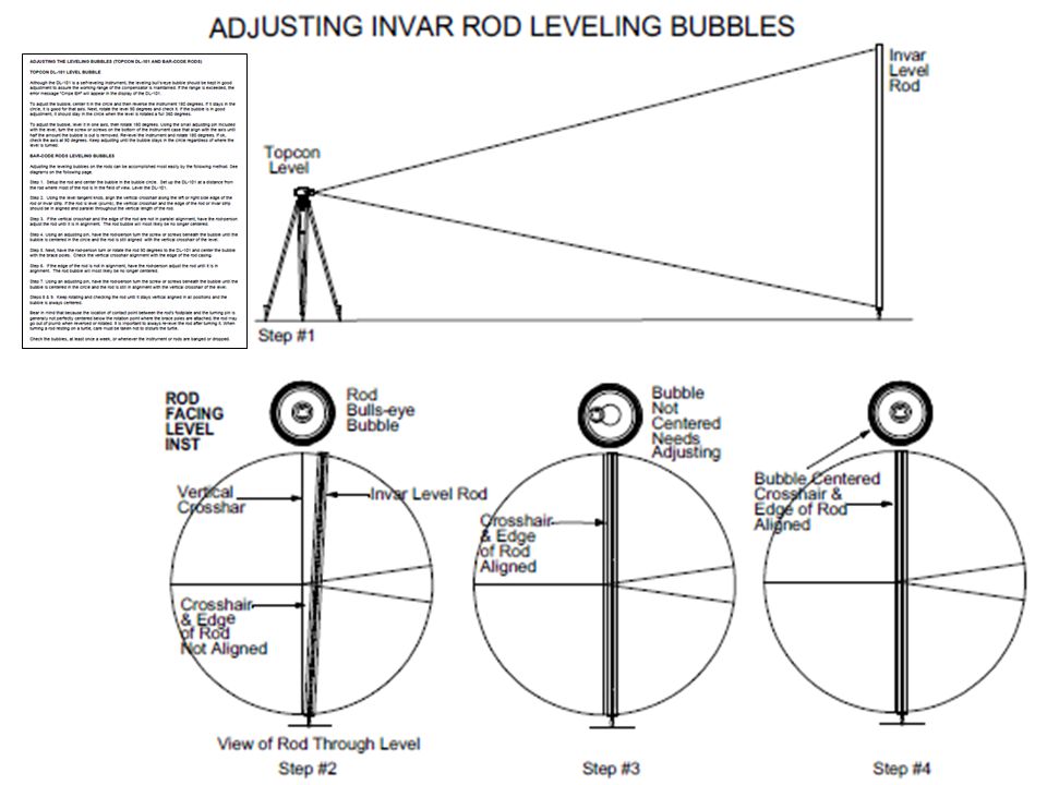


TOOLS TO OBTAIN GEODETIC CONTROL.>")


 and the Defense Mapping School Reviewed by:____________ Date:_________ Objective:>")


