Download presentation
Presentation is loading. Please wait.

1
電腦視覺 Computer and Robot Vision I Chapter2: Binary Machine Vision: Thresholding and Segmentation Instructor: Shih-Shinh Huang 1

2
Contents Introduction Thresholding Connected Components Labeling Signature Segmentation and Analysis 2

3
Computer and Robot Vision I 2.1 Introduction Introduction 3

4
Binary Machine Vision Binary Image Binary Value 1: Part of Object Binary Value 0: Background Pixel Definition of Binary Machine Vision Generation and analysis of such a binary image 2.1 Introduction 4

5
Binary Machine Vision Thresholding It is the first step of binary machine vision It is a labeling operation Connected Components / Signature Analysis They are multilevel vision grouping techniques. They make a transformation from image pixels to more complex units. Regions Segments 2.1 Introduction 5

6
Computer and Robot Vision I 2.2 Thresholding Introduction 6

7
What is Thresholding ? It is a labeling operation. It assigns a binary value to each pixel. Binary Value 1: pixels have higher intensity values Binary Value 0: pixels have higher intensity values 2.2 Thresholding 7

8
Introduction Mathematical Formulation : row and column : gray-level intensity image : intensity threshold : binary intensity image 8 2.2 Thresholding

9
Introduction 9 2.2 Thresholding How to select an appropriate threshold ?

10
Introduction Approaches Global Thresholding: use a global value to make the pixel distinction in the image. Local Thresholding: use spatial varying threshold to label the local pixels. 10 2.2 Thresholding Image

11
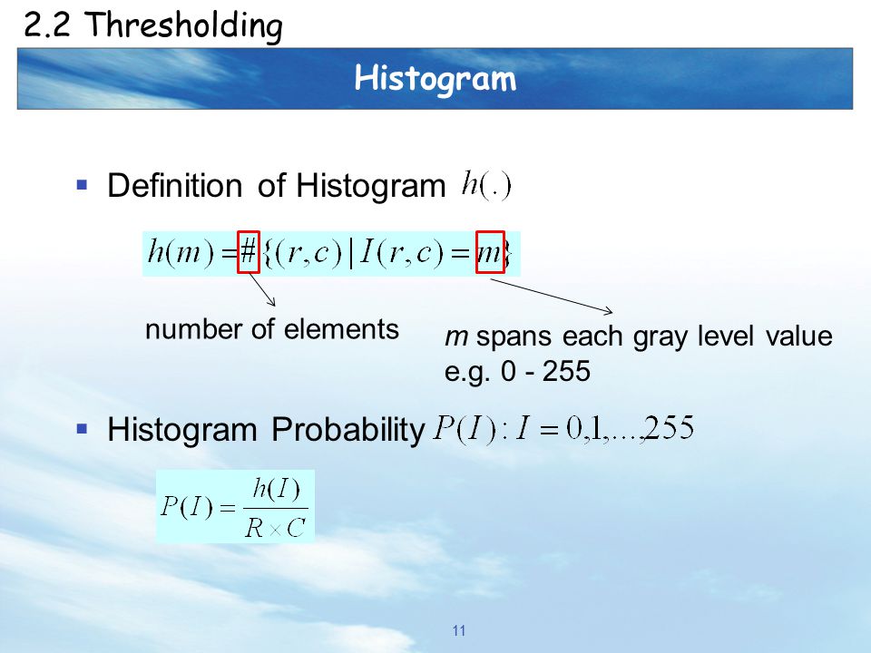
Histogram Definition of Histogram Histogram Probability 11 2.2 Thresholding number of elements m spans each gray level value e.g. 0 - 255
12
Histogram Examples 12 2.2 Thresholding

13
Histogram 13 2.2 Thresholding

14
Histogram 14 2.2 Thresholding T=110T=130T=150T=170

15
Within-Group Variance Observations A group is a set of pixels with intensity homogeneity. Homogeneity is measured by the use of variance High homogeneity group has low variance Low homogeneity group has high variance Objective Select a dividing score such that the weighted sum of the within-group variances is minimized. 15 2.2 Thresholding

16
Within-Group Variance Definition: weighted sum of group variances : probability for the group with values : variance for the group with values 16 2.2 Thresholding

17
Within-Group Variance Objective Formulation Find a threshold which minimizes 17 2.2 Thresholding

18
Within-Group Variance Implementation Issue Step1: For t=0,…,255 Step2: Compute,,, and Step3: Compute Step4: If is less than the value in the previous iteration 18 2.2 Thresholding All variables should be re-compute at each iteration.

19
Within-Group Variance Implementation Issue Speed-Up Formulation 19 2.2 Thresholding

20
Within-Group Variance Implementation Issue Speed-Up Formulation 20 2.2 Thresholding

21
Within-Group Variance Implementation Issue Speed-Up Formulation 21 2.2 Thresholding

22
Within-Group Variance Implementation Issue Speed-Up Formulation 22 2.2 Thresholding

23
Within-Group Variance Implementation Issue Speed-Up Formulation 23 2.2 Thresholding constant minimizemaximize

24
Within-Group Variance Implementation Issue Speed-Up Formulation We have recursive form to compute optimal threshold. 24 2.2 Thresholding

25
Within-Group Variance Example 25 2.2 Thresholding

26
Kullback Information Distance Assumption The observations come from a weighted mixture of two Gaussians distributions. Gaussian Distribution of Background Gaussian Distribution of Object 26 2.2 Thresholding

27
Kullback Information Distance 27 2.2 Thresholding Background Gaussian Distribution Object Gaussian Distribution

28
Kullback Information Distance Objective Formulation T Determine a threshold T that results in two Gaussian distributions which minimize Kullback divergence P(I) :P(I) : observed histogram distribution f(I) Tf(I) : a mixture of Gaussian distributions determined by T 28 2.2 Thresholding
 :P(I) : observed histogram distribution f(I) Tf(I) : a mixture of Gaussian distributions determined by T Thresholding")
29
Kullback Information Distance Objective Formulation Known Parameter: Observed Histogram Unknown Parameter: Two Gaussian Distributions 29 2.2 Thresholding

30
Kullback Information Distance Solution Derivation 30 2.2 Thresholding Constant

31
Kullback Information Distance Solution Derivation Assumption: The modes are well separated. 31 2.2 Thresholding

32
Kullback Information Distance Solution Derivation 32 2.2 Thresholding

33
Kullback Information Distance Implementation Issue Step1: For t=0,…,255 Step2: Compute,,, and Step3: Compute Step4: If is less than the value in the previous iteration 33 2.2 Thresholding

34
Kullback Information Distance Example 34 2.2 Thresholding

35
Kullback Information Distance 35 2.2 Thresholding Within Group Variance (Otsu) Kullback Information (Kittler-Illingworth)
 Kullback Information (Kittler-Illingworth)")
36
Computer and Robot Vision I 2.3 Connected Component Labeling Introduction 36

37
Introduction Description Connected Components labeling is a grouping operation. It performs the unit change from pixel to region or segment. All pixels are given the same identifier Have value binary 1 Connect to each other 37 2.3 Connected Component Labeling

38
Introduction Terminology label: unique name or index of the region connected components labeling: a grouping operation pixel property: position, gray level or brightness level region property: shape, bounding box, position, intensity statistics 38 2.3 Connected Component Labeling

39
Connected Component Operators Definition of Connected Component Two pixels and belong to the same connected component if there is a sequence of 1-pixels, where are neighbor 39 2.3 Connected Component Labeling

40
Connected Component Operators Neighborhood Types 40 2.3 Connected Component Labeling 4-connected 8-connected Original ImageConnected Components

41
Connected Component Algorithms Common Features Process a row of image at a time Assign a new labels to the first pixel of each component. Propagate the label of a pixel to its neighbors to the right or below it. 41 2.3 Connected Component Labeling

42
Connected Component Algorithms Common Features 42 2.3 Connected Component Labeling What label should be assigned to A How does the algorithm keep track of the equivalence of two labels How does the algorithm use the equivalence information to complete the processing

43
Algorithm1: Iterative Algorithm Algorithm Steps Step1 (Initialization): Assign an unique label to each pixel. Step2 (Iteration) : Perform a sequence of top- down and bottom-up label propagation. 43 2.3 Connected Component Labeling Use no auxiliary storage Computational Expensive
 : Perform a sequence of top- down and bottom-up label propagation Connected Component Labeling Use no auxiliary storage Computational Expensive.")
44
Algorithm2: Classic Algorithm Two-Pass Algorithm Pass 1: Perform label assignment and label propagation Construct the equivalence relations between labels when two different labels propagate to the same pixel. Apply resolve function to find the transitive closure of all equivalence relations. Pass 2: Perform label translation. 44 2.3 Connected Component Labeling

45
Algorithm2: Classic Algorithm Example: 45 2.3 Connected Component Labeling {2=4} {3=5} {1=5}

46
Algorithm2: Classic Algorithm Example: Resolve Function 46 2.3 Connected Component Labeling {2=4}{3=5}{1=5}{2=4}{1=3=5} Computational Efficiency Need a lot of space to store equivalence

47
Computer and Robot Vision I 2.4 Signature Segmentation and Analysis Introduction 47

48
Introduction Description Signature analysis perform unit change from the pixel to the segment. It was firstly used in character recognition Definition of Signature The signature, which is a projection, is the histogram of the non-zero pixels of the masked image. 48 2.4 Signature Segmentation and Analysis

49
Introduction General Signatures Vertical Projection Horizontal Projection Diagonal Projection 49 2.4 Signature Segmentation and Analysis

50
Signature Segmentation Steps Thresholding : generate the binary image. Projection Computation: compute the vertical, horizontal, or diagonal projections. Projection Segmentation: divide the image into several segments or regions according to the signatures. 50 2.4 Signature Segmentation and Analysis

51
Signature Segmentation 51 2.4 Signature Segmentation and Analysis

52
Signature Segmentation 52 2.4 Signature Segmentation and Analysis

53
Signature Segmentation 53 2.4 Signature Segmentation and Analysis OCR: Optical Character Recognition MICR: Magnetic Ink Character Recognition

54
The End Computer and Robot Vision I

Similar presentations


 2 0 represents the background 1 represents the foreground 00010010001000 00011110001000 00010010001000.>")