1. Potential vorticity and the dynamic tropopause
John R. Gyakum
Department of Atmospheric and Oceanic Sciences
McGill University
Phone:

2. Outline Motivation (why use potential vorticity??)
Isentropic coordinates
Potential vorticity structures
Potential vorticity invertability
Dynamic tropopause analyses
Comparison of potential vorticity analyses with traditional quasi-geostrophic analyses

3. Motivation (why use potential vorticity
Motivation (why use potential vorticity??) PV = g(-q/p)zaq g is gravity, zaq is the component of absolute vorticity normal to an isentropic surface, and -q/p is the static stability
It is conserved in adiabatic, frictionless three-dimensional flow

4. Consider the following animation of PV on the 325 potential temperature surface:

6. What are the units of PV? PV = g(-q/p)zaq
typical tropospheric values:
-q/p = 10K/100 hPa
zaq≈f=10-4 s-1
and
PV=10 m s-2(10K/100 hPa)(1 hPa(100 kg m s-2m-2)-1)10-4s -1
=10-6 m2 s -1 K kg-1= 1.0 Potential Vorticity Unit (PVU)
Values of PV less than 1.5 PVUs are typically associated with tropospheric air and values greater than 1.5 PVUs are typically associated with stratospheric air

7. Now, we are prepared to
appreciate the cross sections
that we viewed at the end of
this morning’s lecture!
1 PVU= 10-6 m2 s-1K kg-1
The shaded zone illustrates that the
1-3PVU band lies within the
transition zone between the upper
troposphere’s weak stratification
and the relatively strong stratifica-
tion of the lower stratosphere
(Morgan and Nielsen-Gammon
1998).

8. Non-conservation of PV is often associated with interesting diabatic effects in explosive cyclones (Dickinson et al. 1997)

9. Isentropic coordinates (potential temperature is the vertical coordinate)
Air parcels will conserve potential temperature for isentropic processes
Vertical motions can be visualized
moisture transports can be better visualized than on pressure surfaces
Isentropic surfaces can be used to diagnose potential vorticity

10. potential temperature cross section: isentropes slope up to cold air
Consider the comparison of the cross sections we have been viewing: temperature cross section
potential temperature cross
section:
isentropes slope up to cold air
and downward to warm air
high/low pressure on a theta
surface corresponds to warm/
cold temperature on a pressure
surface

11. 292 K Montgomery stream function
((m2 s-2 /100) solid) and pressure
(hPa; dashed)
700 hPa heights (m; solid) and
Temperature (K; dashed)

12. Potential vorticity structures
surface cyclone
surface anticyclone
upper-tropospheric trough
upper-tropospheric ridge

13. Surface cyclone (warm ‘anomaly’) PV = g(-q/p)zaq
warm air is associated with isentropes becoming packed near the ground (more PV)
surface cyclone is associated with a warm core with no disturbance aloft (zT= zgu- zgl=0-zgl<0
200
Pressure
(hPa)
cold
warm
more stable
cold
1000
distance (km)

14. Surface anticyclone (cold ‘anomaly’) PV = g(-q/p)zaq
cold air is associated with isentropes becoming less packed near the ground (less PV and smaller static stability)
surface anticyclone is associated with a cold core with no disturbance aloft (zT= zgu- zgl=0-zgl>0
200
Pressure
(hPa)
warm
cold
less stable
warm
1000
distance (km)

15. Upper-tropospheric trough (positive PV ‘anomaly’) PV = g(-q/p)zaq
cold tropospheric air is associated with isentropes becoming more packed near the tropopause (more PV and greater static stability)
upper tropospheric trough is associated with a cold core cyclone with no disturbance below (zT= zgu- zgl= zgu-0>0
200
warm
more
stable
cold
cold
Pressure
(hPa)
warm
warm
cold
less stable
1000
distance (km)

16. Upper-tropospheric ridge (negative PV ‘anomaly’) PV = g(-q/p)zaq
warm tropospheric air is associated with isentropes becoming less packed near the tropopause (less PV and smaller static stability)
upper tropospheric ridge is associated with a warm core anticyclone with no disturbance below (zT= zgu- zgl= zgu-0<0
200
warm
warm
cold
Pressure
(hPa)
less stable
warm
more
stable
cold
cold
1000
distance (km)

17. Potential vorticity invertability
If we know the distribution of isentropic potential vorticity, then we also know the wind field
The wind field is ‘induced’ by the PV anomaly field
The amplitude of the induced wind increases with size of the anomaly and with a reduction in static stability

18. Potential vorticity inversion may be used to understand the motions of troughs and ridges:
Potential vorticity maxima and minima
instantaneous winds
max min max min N

19. Consider a PV reference state:
Consider the PV contours at right with increasing PV northward (owing primarily to increase of the Coriolis parameter)
larger PV
PV+2dPV N
PV+dPV PV
PV-dPV

20. Consider the introduction of alternating PV anomalies:
The sense of the wind field that is induced by the PV anomalies
There will be a propagation to the left or to the west (largest effecct for large anomalies
This effect is opposed by the eastward advective effect
larger PV N
PV+2dPV L + -
PV+dPV + PV
East

21. The application of PV inversion to the problem of cyclogenesis (Hoskins et al. 1985)

22. Dynamic tropopause analysis; What is the dynamic tropopause?
A level (not at a constant height or pressure) at which the gradients of potential vorticity on an isentropic surface are maximized
Large local changes in PV are determined by the advective wind
This level ranges from 1.5 to 3.0 Potential vorticity units (PVUs)

23. Consider the cross sections that we have been viewing:
Our focus is on the isentropic cross section seen below
the opposing slopes of the PV surfaces and the isentropes result in the gradients of PV being sharper along isentropic surfaces than along isobaric surfaces

26. Dynamic tropopause pressure: A
Relatively high (low pressure)
Tropopause in the subtropics, and a
Relatively low (high pressure)
Tropopause in the polar regions; a
Steeply-sloping tropopause in the
Middle latitudes

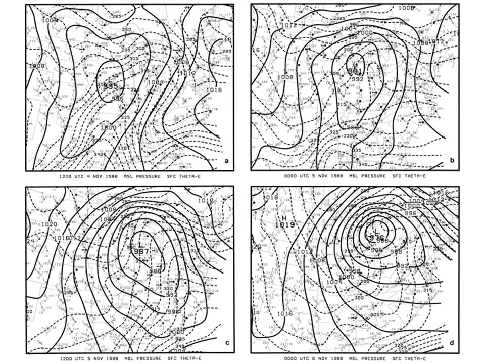
29. Tropopause potential
temperatures (contour interval
of 5K from 305 K to 350 K) at
12-h intervals (from Morgan and
Nielsen-Gammon 1998)
The appearance of the 330 K
closed contour in panel c is
produced by the large values of
equivalent potential temperature
ascending in moist convection
and ventilated at the tropopause
level;
as discussed earlier, this is an
excellent means of showing the
effects of diabatic heating, and
verifying models

30. the sounding shows a tropopause
fold extending from 500 to 375
hPa at 1200 UTC, 5 Nov. 1988
for Centerville, AL,
with tropospheric air above and
extending to 150 hPa.
The fold has descended into
Charleston, SC by 0000 UTC,
6 November 1988 to the
hPa layer. The same isentropic
levels are associated with each fold

31. Coupling index:
Theta at the tropopause
Minus the equivalent
Potential temperature at
Low levels
(a poor man’s lifted index)

32. December 30-31, 1993 SLP
And 925 hPa theta

39. An example illustrates the detail of the dynamic tropopause (1
An example illustrates the detail of the dynamic tropopause (1.5 potential vorticity units) that is lacking in a constant pressure analysis

40. 250 and 500-hPa analyses showing the respective subtropical and polar jets:
250-hPa z and winds
500-hPa z and winds

41. Dynamic tropopause map shows the properly-sharp troughs and ridges and full amplitudes of both the polar and subtropical jets

45. The dynamic tropopause animation during the 11 May 1999 hailstorm:

47. An animation of the dynamic tropopause for the period from December 1, 1998 through February 28, 1999:

49. Comparison of potential vorticity analyses with traditional quasi-geostrophic analyses
Focus is on the PV perspective of QG vertical motions and the movement of high and low pressure systems

50. OK, but what about PV????
Consider a positive PV anomaly (PV maximum) aloft in a westerly shear flow: z
+ PV anomaly x

51. Now, consider a reference frame of the PV anomaly in which the anomaly is fixed:
Consider the quasi-geostrophic
Vorticity equation in the reference
Frame of the positive PV anomaly
0= -vg(g + f)-f0 z
+ PV anomaly
>0
<0
AVA; <0
CVA; >0 x

52. Now, consider the same PV anomaly in which the anomaly is fixed from the perspective of the thermodynamic equation: z
+ PV anomaly
0 = -vg  T + ws(p/R)
cool x z
+ PV anomaly
cool
>0
<0 CA WA x

53. Consider vertical motions in the vicinity of a warm surface potential temperature anomaly (surrogate PV anomaly) from the vorticity equation:
0= -vg(g + f)-f0 z
CVA
>0
AVA
<0
>0
<0 x
+ PV +

54. Consider vertical motions in the vicinity of a warm surface potential temperature anomaly (surrogate PV anomaly) from the thermodynamic equation:
0 = -vg  T + ws(p/R) z
cold
<0 y
>0 WA CA
warm
+ PV +

55. Movement of surface cyclones and anticyclones on level terrain:
Consider a reference state of potential temperature:
North
 -   
 +  

56. Consider that air parcels are displaced alternately poleward and equatorward within the east-west channel. Potential temperature is conserved for isentropic processes
Since =0 at the surface, potential temperature changes
Occur due to advection only
 -  
North - + 
L/4
L/4
 +  

57. The previous slide shows the maximum cold advection occurs one quarter of a wavelength east of cold potential temperature anomalies, with maximum warm advection occurring one-quarter of a wavelength east of the warm potential temperature anomalies. The entire wave travels (propagates), with the cyclones and anticyclones propagates eastward.
Just as with traditional quasi-geostrophic theory, surface cyclones
Travel from regions of cold advection to regions of warm advection.
Surface anticyclones travel from regions of warm advection to regions
Of cold advection.

58. Orographic effects on the motions of surface cyclones and anticyclones
Consider a statically stable reference state in the vicinity of mountains as shown below, with no relative vorticity on a potential
Temperature surface z
 +   
 -   x

59. Note that cyclones and anticyclones move with higher terrain to their right, in the absence of any other effects.
 +  
 -    N - +
Mountain
Range

60. References
Bluestein, H. B., 1993: Synoptic-dynamic meteorology in midlatitudes. Volume II: Observations and theory of weather systems. Oxford University Press pp.
Dickinson, M. J., and coauthors, 1997: The Marcch 1993 superstorm cyclogenesis: Incipient phase synoptic- and convective-scale flow interaction and model performance. Mon. Wea. Rev., 125,
Hoskins, B. J., M. McIntyre, and A. Robertson, 1985: On the use and significance of isentropic potential vorticity maps. Quart. J. Roy. Meteor. Soc., 111,
Morgan, M. C., and J. W. Nielsen-Gammon, 1998: Using tropopause maps to diagnose midlatitude weather systems. Mon. Wea. Rev., 126,