1. Data and Computer Communications
Chapter 3 – Data Transmission
“Data and Computer Communications”, 9/e, by William Stallings, Chapter 3 “Data Transmission”.
Ninth Edition
by William Stallings
Data and Computer Communications, Ninth Edition by William Stallings, (c) Pearson Education - Prentice Hall, 2011
Data and Computer Communications, Ninth Edition by William Stallings, (c) Pearson Education - Prentice Hall, 2011

2. Data Transmission quality of the signal being transmitted
characteristics of the transmission medium
The successful transmission of data depends on two factors:
The successful transmission of data depends principally on two factors: the quality of the signal being transmitted and the characteristics of the transmission medium. The objective of this chapter and the next is to provide the reader with an intuitive feeling for the nature of these two factors.
Data and Computer Communications, Ninth Edition by William Stallings, (c) Pearson Education - Prentice Hall, 2011

3. Transmission Terminology
Data transmission occurs between transmitter and receiver over some transmission medium.
Communication is in the form of electromagnetic waves.
Guided media
twisted pair, coaxial cable, optical fiber
Unguided media (wireless)
air, vacuum, seawater
In this section we introduce some concepts and terms that will be referred to throughout the rest of the chapter and, indeed, throughout Part Two.
Transmission Terminology
Data transmission occurs between transmitter and receiver over some transmission medium. Transmission media may be classified as guided or unguided. In both cases, communication is in the form of electromagnetic waves. With guided media, the waves are guided along a physical path; examples of guided media are twisted pair, coaxial cable, and optical fiber. Unguided media, also called wireless, provide a means for transmitting electromagnetic waves but do not guide them; examples are propagation through air, vacuum, and seawater.
Data and Computer Communications, Ninth Edition by William Stallings, (c) Pearson Education - Prentice Hall, 2011

4. Transmission Terminology
no intermediate devices
Direct link
direct link
only 2 devices share link
Point-to-point
more than two devices share the link
Multi-point
The term direct link is used to refer to the transmission path between two devices in which signals propagate directly from transmitter to receiver with no intermediate devices, other than amplifiers or repeaters used to increase signal strength. Note that this term can apply to both guided and unguided media.
A guided transmission medium is point to point if it provides a direct link between two devices and those are the only two devices sharing the medium. In a multipoint guided configuration, more than two devices share the same medium.
Data and Computer Communications, Ninth Edition by William Stallings, (c) Pearson Education - Prentice Hall, 2011

5. Transmission Terminology
Simplex
signals transmitted in one direction
eg. Television
Half duplex
both stations transmit, but only one at a time
eg. police radio
Full duplex
simultaneous transmissions
eg. telephone
A transmission may be simplex, half duplex, or full duplex. In simplex transmission, signals are transmitted in only one direction; one station is transmitter and the other is receiver. In half-duplex operation, both stations may transmit, but only one at a time. In full-duplex operation, both stations may transmit simultaneously. In the latter case, the medium is carrying signals in both directions at the same time. How this can be is explained in due course.
We should note that the definitions just given are the ones in common use in the United States (ANSI definitions). Elsewhere (ITU-T definitions), the term simplex is used to correspond to half duplex as defined previously, and duplex is used to correspond to full duplex as just defined.
Data and Computer Communications, Ninth Edition by William Stallings, (c) Pearson Education - Prentice Hall, 2011

6. Frequency, Spectrum and Bandwidth
Time Domain Concepts
analog signal
signal intensity varies smoothly with no breaks
digital signal
signal intensity maintains a constant level and then abruptly changes to another level
periodic signal
signal pattern repeats over time
aperiodic signal
pattern not repeated over time
Frequency, Spectrum, and Bandwidth
In this book, we are concerned with electromagnetic signals used as a means to transmit data. At point 3 in Stallings DCC9e Figure 1.5, a signal is generated by the transmitter and transmitted over a medium. The signal is a function of time, but it can also be expressed as a function of frequency; that is, the signal consists of components of different frequencies. It turns out that the frequency domain view of a signal is more important to an understanding of data transmission than a time domain view. Both views are introduced here.
Time Domain Concepts
Viewed as a function of time, an electromagnetic signal can be either analog or digital. An analog signal is one in which the signal intensity varies in a smooth, or continuous, fashion over time. In other words, there are no breaks or discontinuities in the signal. A digital signal is one in which the signal intensity maintains a constant level for some period of time and then abruptly changes to another constant level, in a discrete fashion. Stalling DCC9e Figure 3.1 shows an example of each kind of signal. The analog signal might represent speech, and the digital signal might represent binary 1s and 0s.
The simplest sort of signal is a periodic signal, in which the same signal pattern repeats over time. Stallings DDC9e Figure 3.2 shows an example of a periodic continuous signal (sine wave) and a periodic discrete signal (square wave). Mathematically, a signal s(t) is defined to be periodic if and only if
s(t + T) = s(t) –∞ < t < +∞
where the constant T is the period of the signal (T is the smallest value that satisfies the equation). Otherwise, a signal is aperiodic.
A mathematical definition: a signal s(t) is continuous if for all a.
This is an idealized definition. In fact, the transition from one voltage level to another will not be instantaneous, but there will be a small transition period. Nevertheless, an actual digital signal approximates closely the ideal model of constant voltage levels with instantaneous transitions.
Data and Computer Communications, Ninth Edition by William Stallings, (c) Pearson Education - Prentice Hall, 2011

7. Analog and Digital Signals
Stallings DCC9e Figure 3.1 shows an example of both analog or digital signals. The continuous signal might represent speech, and the discrete signal might represent binary 1s and 0s.
Data and Computer Communications, Ninth Edition by William Stallings, (c) Pearson Education - Prentice Hall, 2011

8. Periodic Signals
The simplest sort of signal is a periodic signal, in which the same signal pattern repeats over time.
In Stallings DCC9e Figure 3.2 a signal is generated by the transmitter and transmitted over a medium. The signal is a function of time, but it can also be expressed as a function of frequency; that is, the signal consists of components of different frequencies. It turns out that the frequency domain view of a signal is more important to an understanding of data transmission than a time domain view. Both views are introduced here.
Data and Computer Communications, Ninth Edition by William Stallings, (c) Pearson Education - Prentice Hall, 2011

9. Sine Wave (periodic continuous signal) peak amplitude (A)
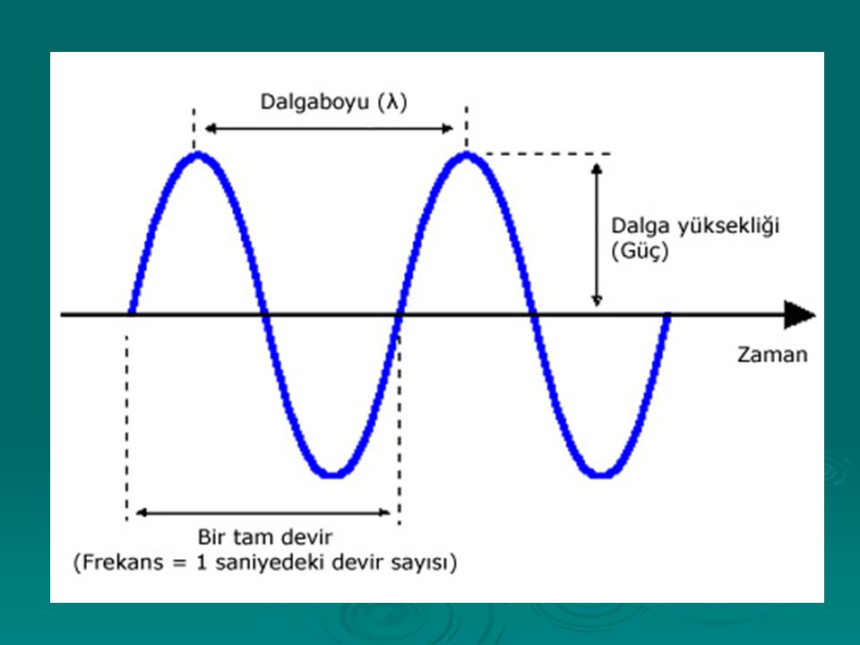
maximum strength of signal
typically measured in volts
frequency (f)
rate at which the signal repeats
Hertz (Hz) or cycles per second
period (T) is the amount of time for one repetition
T = 1/f
phase ()
relative position in time within a single period of signal
The sine wave is the fundamental periodic signal. A general sine wave can be represented by three parameters: peak amplitude (A), frequency (f), and phase (f). The peak amplitude is the maximum value or strength of the signal over time; typically, this value is measured in volts. The frequency is the rate [in cycles per second, or hertz (Hz)] at which the signal repeats. An equivalent parameter is the period (T) of a signal, which is the amount of time it takes for one repetition; therefore, T = 1/f. Phase is a measure of the relative position in time within a single period of a signal, as is illustrated subsequently. More formally, for a periodic signal f(t), phase is the fractional part t/T of the period T through which t has advanced relative to an arbitrary origin. The origin is usually taken as the last previous passage through zero from the negative to the positive direction.
Data and Computer Communications, Ninth Edition by William Stallings, (c) Pearson Education - Prentice Hall, 2011

10. Varying Sine Waves s(t) = A sin(2ft +)
The general sine wave can be written
s(t) = A sin(2πft + f)
A function with the form of the preceding equation is known as a sinusoid. Stallings DCC9e Figure 3.3 shows the effect of varying each of the three parameters. In part (a) of the figure, the frequency is 1 Hz; thus the period is T = 1 second. Part (b) has the same frequency and phase but a peak amplitude of 0.5. In part (c) we have f = 2, which is equivalent to T = 0.5. Finally, part (d) shows the effect of a phase shift of π/4 radians, which is 45 degrees (2π radians = 360˚ = 1 period).
In Stallings DCC9e Figure 3.3, the horizontal axis is time; the graphs display the value of a signal at a given point in space as a function of time. These same graphs, with a change of scale, can apply with horizontal axes in space. In this case, the graphs display the value of a signal at a given point in time as a function of distance. For example, for a sinusoidal transmission (e.g., an electromagnetic radio wave some distance from a radio antenna, or sound some distance from a loudspeaker), at a particular instant of time, the intensity of the signal varies in a sinusoidal way as a function of distance from the source.
Data and Computer Communications, Ninth Edition by William Stallings, (c) Pearson Education - Prentice Hall, 2011

11. the wavelength of a signal is the distance occupied by a single cycle
can also be stated as the distance between two points of corresponding phase of two consecutive cycles
assuming signal velocity v, then the wavelength is related to the period as  = vT
or equivalently f = v
especially when v=c
c = 3*108 ms-1 (speed of light in free space)
There is a simple relationship between the two sine waves, one in time and one in space. The wavelength () of a signal is the distance occupied by a single cycle, or, put another way, the distance between two points of corresponding phase of two consecutive cycles. Assume that the signal is traveling with a velocity v. Then the wavelength is related to the period as follows: l = vT. Equivalently, lf = v. Of particular relevance to this discussion is the case where v = c, the speed of light in free space, which is approximately 3 ´ 108 m/s.
Data and Computer Communications, Ninth Edition by William Stallings, (c) Pearson Education - Prentice Hall, 2011

13. Frequency Domain Concepts
signals are made up of many frequencies
components are sine waves
Fourier analysis can show that any signal is made up of components at various frequencies, in which each component is a sinusoid
can plot frequency domain functions
Frequency Domain Concepts
In practice, an electromagnetic signal will be made up of many frequencies. For example, the signal
s(t) = [(4/π)  (sin(2πft) + (1/3) sin(2π(3f)t)]
is shown in Stallings DCC9e Figure 3.4c. The components of this signal are just sine waves of frequencies f and 3f; parts (a) and (b) of the figure show these individual components. There are two interesting points that can be made about this figure:
The second frequency is an integer multiple of the first frequency. When all of the frequency components of a signal are integer multiples of one frequency, the latter frequency is referred to as the fundamental frequency. Each multiple of the fundamental frequency is referred to as a harmonic frequency of the signal.
The period of the total signal is equal to the period of the fundamental frequency. The period of the component sin (2πft) is T = 1/f, and the period of s(t) is also T, as can be seen from Figure 3.4c.
It can be shown, using a discipline known as Fourier analysis, that any signal is made up of components at various frequencies, in which each component is a sinusoid. By adding together enough sinusoidal signals, each with the appropriate amplitude, frequency, and phase, any electromagnetic signal can be constructed. Put another way, any electromagnetic signal can be shown to consist of a collection of periodic analog signals (sine waves) at different amplitudes, frequencies, and phases. The importance of being able to look at a signal from the frequency perspective (frequency domain) rather than a time perspective (time domain) should become clear as the discussion proceeds. For the interested reader, the subject of Fourier analysis is introduced in Appendix A.
Data and Computer Communications, Ninth Edition by William Stallings, (c) Pearson Education - Prentice Hall, 2011

14. Addition of Frequency Components (T=1/f)
c is sum of f & 3f
In Stallings DCC9e Figure 3.4c, the components of this signal are just sine waves of frequencies f and 3f, as shown in parts (a) and (b).
Data and Computer Communications, Ninth Edition by William Stallings, (c) Pearson Education - Prentice Hall, 2011

15. Data Rate and Bandwidth
any transmission system has a limited band of frequencies
this limits the data rate that can be carried on the transmission medium
square waves have infinite components and hence an infinite bandwidth
most energy in first few components
limiting bandwidth creates distortions
Relationship between Data Rate and Bandwidth
We have said that effective bandwidth is the band within which most of the signal energy is concentrated. The meaning of the term most in this context is somewhat arbitrary. The important issue here is that, although a given waveform may contain frequencies over a very broad range, as a practical matter any transmission system (transmitter plus medium plus receiver) will be able to accommodate only a limited band of frequencies. This, in turn, limits the data rate that can be carried on the transmission medium.
To try to explain these relationships, consider the square wave of Stallings DCC9e Figure 3.2b. Suppose that we let a positive pulse represent binary 0 and a negative pulse represent binary 1. Then the waveform represents the binary stream 0101…. The duration of each pulse is 1/(2f); thus the data rate is 2f bits per second (bps). What are the frequency components of this signal? To answer this question, consider again Stallings DCC9e Figure 3.4. By adding together sine waves at frequencies f and 3f, we get a waveform that begins to resemble the original square wave. Let us continue this process by adding a sine wave of frequency 5f, as shown in Stallings DCC9e Figure 3.7a, and then adding a sine wave of frequency 7f, as shown in Stallings DCC9e Figure 3.7b. As we add additional odd multiples of f, suitably scaled, the resulting waveform approaches that of a square wave more and more closely.
Thus, this waveform has an infinite number of frequency components and hence an infinite bandwidth. However, the peak amplitude of the kth frequency component, kf, is only 1/k, so most of the energy in this waveform is in the first few frequency components. What happens if we limit the bandwidth to just the first three frequency components? We have already seen the answer, in Stallings DCC9e Figure 3.7a. As we can see, the shape of the resulting waveform is reasonably close to that of the original square wave.
We can draw the following conclusions from the preceding example. In general, any digital waveform will have infinite bandwidth. If we attempt to transmit this waveform as a signal over any medium, the transmission system will limit the bandwidth that can be transmitted. Furthermore, for any given medium, the greater the bandwidth transmitted, the greater the cost. Thus, on the one hand, economic and practical reasons dictate that digital information be approximated by a signal of limited bandwidth. On the other hand, limiting the bandwidth creates distortions, which makes the task of interpreting the received signal more difficult. The more limited the bandwidth, the greater the distortion, and the greater the potential for error by the receiver.
One more illustration should serve to reinforce these concepts. Stallings DCC9e Figure 3.8 shows a digital bit stream with a data rate of 2000 bits per second. With a bandwidth of 2500 Hz, or even 1700 Hz, the representation is quite good. Furthermore, we can generalize these results. If the data rate of the digital signal is W bps, then a very good representation can be achieved with a bandwidth of 2W Hz. However, unless noise is very severe, the bit pattern can be recovered with less bandwidth than this (see the discussion of channel capacity in Section 3.4).
Thus, there is a direct relationship between data rate and bandwidth: the higher the data rate of a signal, the greater is its required effective bandwidth. Looked at the other way, the greater the bandwidth of a transmission system, the higher is the data rate that can be transmitted over that system.
Another observation worth making is this: If we think of the bandwidth of a signal as being centered about some frequency, referred to as the center frequency, then the higher the center frequency, the higher the potential bandwidth and therefore the higher the potential data rate. For example, if a signal is centered at 2 MHz, its maximum potential bandwidth is 4 MHz.
We return to a discussion of the relationship between bandwidth and data rate in Section 3.4, after a consideration of transmission impairments.
There is a direct relationship between
data rate and bandwidth.
Data and Computer Communications, Ninth Edition by William Stallings, (c) Pearson Education - Prentice Hall, 2011

16. Analog and Digital Data Transmission
entities that convey information
signals
electric or electromagnetic representations of data
signaling
physically propagates along a medium
transmission
communication of data by propagation and processing of signals
The terms analog and digital correspond, roughly, to continuous and discrete, respectively. These two terms are used frequently in data communications in at least three contexts: data, signaling, and transmission.
Briefly, we define data as entities that convey meaning, or information. Signals are electric or electromagnetic representations of data. Signaling is the physical propagation of the signal along a suitable medium. Transmission is the communication of data by the propagation and processing of signals. In what follows, we try to make these abstract concepts clear by discussing the terms analog and digital as applied to data, signals, and transmission.
Data and Computer Communications, Ninth Edition by William Stallings, (c) Pearson Education - Prentice Hall, 2011

17. Acoustic Spectrum (Analog)
The most familiar example of analog data is audio, which, in the form of acoustic sound waves, can be perceived directly by human beings. Stallings DCC9e Figure 3.9 shows the acoustic spectrum for human speech and for music. Frequency components of typical speech may be found between approximately 100 Hz and 7 kHz. Although much of the energy in speech is concentrated at the lower frequencies, tests have shown that frequencies below 600 or 700 Hz add very little to the intelligibility of speech to the human ear. Typical speech has a dynamic range of about 25 dB; that is, the power produced by the loudest shout may be as much as 300 times greater than the least whisper. Stallings DCC9e Figure 3.9 also shows the acoustic spectrum and dynamic range for music.
Another common example of analog data is video. Here it is easier to characterize the data in terms of the TV screen (destination) rather than the original scene (source) recorded by the TV camera. To produce a picture on the screen, an electron beam scans across the surface of the screen from left to right and top to bottom. For black-and-white television, the amount of illumination produced (on a scale from black to white) at any point is proportional to the intensity of the beam as it passes that point. Thus at any instant in time the beam takes on an analog value of intensity to produce the desired brightness at that point on the screen. Further, as the beam scans, the analog value changes. Thus the video image can be thought of as a time-varying analog signal.
Data and Computer Communications, Ninth Edition by William Stallings, (c) Pearson Education - Prentice Hall, 2011

18. Analog and Digital Transmission
Stallings DCC9e Figure 3.10 depicts the scanning process. At the end of each scan line, the beam is swept rapidly back to the left (horizontal retrace). When the beam reaches the bottom, it is swept rapidly back to the top (vertical retrace). The beam is turned off (blanked out) during the retrace intervals.
To achieve adequate resolution, the beam produces a total of 483 horizontal lines at a rate of 30 complete scans of the screen per second. Tests have shown that this rate will produce a sensation of flicker rather than smooth motion. To provide a flicker-free image without increasing the bandwidth requirement, a technique known as interlacing is used. As Stallings DCC9e Figure 3.10 shows, the odd numbered scan lines and the even numbered scan lines are scanned separately, with odd and even fields alternating on successive scans. The odd field is the scan from A to B and the even field is the scan from C to D. The beam reaches the middle of the screen's lowest line after lines. At this point, the beam is quickly repositioned at the top of the screen and recommences in the middle of the screen's topmost visible line to produce an additional lines interlaced with the original set. Thus the screen is refreshed 60 times per second rather than 30, and flicker is avoided.
Data and Computer Communications, Ninth Edition by William Stallings, (c) Pearson Education - Prentice Hall, 2011

19. Advantages & Disadvantages of Digital Signals
cheaper
less susceptible to noise interference
suffer more from attenuation
digital now preferred choice
A digital signal is a sequence of voltage pulses that may be transmitted over a wire medium; for example, a constant positive voltage level may represent binary 0 and a constant negative voltage level may represent binary 1.
The principal advantages of digital signaling are that it is generally cheaper than analog signaling and is less susceptible to noise interference. The principal disadvantage is that digital signals suffer more from attenuation than do analog signals. Stallings DCC9e Figure 3.11 shows a sequence of voltage pulses, generated by a source using two voltage levels, and the received voltage some distance down a conducting medium. Because of the attenuation, or reduction, of signal strength at higher frequencies, the pulses become rounded and smaller. It should be clear that this attenuation can lead rather quickly to the loss of the information contained in the propagated signal.
In what follows, we first look at some specific examples of signal types and then discuss the relationship between data and signals.
Data and Computer Communications, Ninth Edition by William Stallings, (c) Pearson Education - Prentice Hall, 2011

20. Audio Signals frequency range of typical speech is 100Hz-7kHz
easily converted into electromagnetic signals
varying volume converted to varying voltage
can limit frequency range for voice channel to Hz
Let us return to our three examples of the preceding subsection. For each example, we will describe the signal and estimate its bandwidth.
The most familiar example of analog information is audio, or acoustic, information, which, in the form of sound waves, can be perceived directly by human beings. One form of acoustic information, of course, is human speech. This form of information is easily converted to an electromagnetic signal for transmission (Stallings DCC9e Figure 3.12). In essence, all of the sound frequencies, whose amplitude is measured in terms of loudness, are converted into electromagnetic frequencies, whose amplitude is measured in volts. The telephone handset contains a simple mechanism for making such a conversion.
In the case of acoustic data (voice), the data can be represented directly by an electromagnetic signal occupying the same spectrum. However, there is a need to compromise between the fidelity of the sound as transmitted electrically and the cost of transmission, which increases with increasing bandwidth. As mentioned, the spectrum of speech is approximately 100 Hz to 7 kHz, although a much narrower bandwidth will produce acceptable voice reproduction. The standard spectrum for a voice channel is 300 to 3400 Hz. This is adequate for speech transmission, minimizes required transmission capacity, and allows the use of rather inexpensive telephone sets. The telephone transmitter converts the incoming acoustic voice signal into an electromagnetic signal over the range 300 to 3400 Hz. This signal is then transmitted through the telephone system to a receiver, which reproduces it as acoustic sound.
Data and Computer Communications, Ninth Edition by William Stallings, (c) Pearson Education - Prentice Hall, 2011

21. Video Signals to produce a video signal a TV camera is used
USA standard is 483 lines per frame, at a rate of 30 complete frames per second
actual standard is 525 lines but 42 lost during vertical retrace
horizontal scanning frequency is 525 lines x 30 scans = lines per second
max frequency if line alternates black and white
max frequency of 4.2MHz
Video Signals
Now let us look at the video signal. To produce a video signal, a TV camera, which performs similar functions to the TV receiver, is used. One component of the camera is a photosensitive plate, upon which a scene is optically focused. An electron beam sweeps across the plate from left to right and top to bottom, in the same fashion as depicted in Figure 3.10 for the receiver. As the beam sweeps, an analog electric signal is developed proportional to the brightness of the scene at a particular spot. We mentioned that a total of 483 lines are scanned at a rate of 30 complete scans per second. This is an approximate number taking into account the time lost during the vertical retrace interval. The actual U.S. standard is 525 lines, but of these about 42 are lost during vertical retrace. Thus the horizontal scanning frequency is (525 lines)  (30 scan/s) = 15,750 lines per second, or 63.5 µs/line. Of the 63.5 µs, about 11 µs are allowed for horizontal retrace, leaving a total of 52.5 µs per video line.
Now we are in a position to estimate the bandwidth required for the video signal. To do this we must estimate the upper (maximum) and lower (minimum) frequency of the band. We use the following reasoning to arrive at the maximum frequency: The maximum frequency would occur during the horizontal scan if the scene were alternating between black and white as rapidly as possible. We can estimate this maximum value by considering the resolution of the video image. In the vertical dimension, there are 483 lines, so the maximum vertical resolution would be 483. Experiments have shown that the actual subjective resolution is about 70% of that number, or about 338 lines. In the interest of a balanced picture, the horizontal and vertical resolutions should be about the same. Because the ratio of width to height of a TV screen is 4 : 3, the horizontal resolution should be about 4/3 ´ 338 = 450 lines. As a worst case, a scanning line would be made up of 450 elements alternating black and white. The scan would result in a wave, with each cycle of the wave consisting of one higher (black) and one lower (white) voltage level. Thus there would be 450/2 = 225 cycles of the wave in 52.5 µs, for a maximum frequency of about 4.2 MHz. This rough reasoning, in fact, is fairly accurate. The lower limit is a dc or zero frequency, where the dc component corresponds to the average illumination of the scene (the average value by which the brightness exceeds the reference black level). Thus the bandwidth of the video signal is approximately 4 MHz – 0 = 4 MHz.
Data and Computer Communications, Ninth Edition by William Stallings, (c) Pearson Education - Prentice Hall, 2011

22. Conversion of PC Input to Digital Signal
Finally, the third example described is the general case of binary data. Binary data is generated by terminals, computers, and other data processing equipment and then converted into digital voltage pulses for transmission, as illustrated in Stallings DCC9e Figure A commonly used signal for such data uses two constant (dc) voltage levels, one level for binary 1 and one level for binary 0. (In Chapter 5, we shall see that this is but one alternative, referred to as NRZ.) Again, we are interested in the bandwidth of such a signal. This will depend, in any specific case, on the exact shape of the waveform and the sequence of 1s and 0s. We can obtain some understanding by considering Stallings DCC9e Figure 3.8 (compare Figure 3.7). As can be seen, the greater the bandwidth of the signal, the more faithfully it approximates a digital pulse stream.
Data and Computer Communications, Ninth Edition by William Stallings, (c) Pearson Education - Prentice Hall, 2011

23. Digital Signals Data and Signals
In the foregoing discussion, we have looked at analog signals used to represent analog data and digital signals used to represent digital data. Generally, analog data are a function of time and occupy a limited frequency spectrum; such data can be represented by an electromagnetic signal occupying the same spectrum. Digital data can be represented by digital signals, with a different voltage level for each of the two binary digits.
As Stallings DCC9e Figure 3.14 illustrates, these are not the only possibilities. Digital data can also be represented by analog signals by use of a modem (modulator/demodulator). The modem converts a series of binary (two-valued) voltage pulses into an analog signal by encoding the digital data onto a carrier frequency. The resulting signal occupies a certain spectrum of frequency centered about the carrier and may be propagated across a medium suitable for that carrier. The most common modems represent digital data in the voice spectrum and hence allow those data to be propagated over ordinary voice-grade telephone lines. At the other end of the line, another modem demodulates the signal to recover the original data.
In an operation very similar to that performed by a modem, analog data can be represented by digital signals. The device that performs this function for voice data is a codec (coder-decoder). In essence, the codec takes an analog signal that directly represents the voice data and approximates that signal by a bit stream. At the receiving end, the bit stream is used to reconstruct the analog data.
Thus, Stallings DCC9e Figure 3.14 suggests that data may be encoded into signals in a variety of ways. We will return to this topic in Chapter 5.
Data and Computer Communications, Ninth Edition by William Stallings, (c) Pearson Education - Prentice Hall, 2011

24. Analog and Digital Transmission
Both analog and digital signals may be transmitted on suitable transmission media. The way these signals are treated is a function of the transmission system. Stallings DCC9e Table 3.1 summarizes the methods of data transmission. Analog transmission is a means of transmitting analog signals without regard to their content; the signals may represent analog data (e.g., voice) or digital data (e.g., binary data that pass through a modem). In either case, the analog signal will become weaker (attenuate) after a certain distance. To achieve longer distances, the analog transmission system includes amplifiers that boost the energy in the signal. Unfortunately, the amplifier also boosts the noise components. With amplifiers cascaded to achieve long distances, the signal becomes more and more distorted. For analog data, such as voice, quite a bit of distortion can be tolerated and the data remain intelligible. However, for digital data, cascaded amplifiers will introduce errors.
Digital transmission, in contrast, assumes a binary content to the signal. A digital signal can be transmitted only a limited distance before attenuation, noise, and other impairments endanger the integrity of the data. To achieve greater distances, repeaters are used. A repeater receives the digital signal, recovers the pattern of 1s and 0s, and retransmits a new signal. Thus the attenuation is overcome.
The same technique may be used with an analog signal if it is assumed that the signal carries digital data. At appropriately spaced points, the transmission system has repeaters rather than amplifiers. The repeater recovers the digital data from the analog signal and generates a new, clean analog signal. Thus noise is not cumulative.
The question naturally arises as to which is the preferred method of transmission. The answer being supplied by the telecommunications industry and its customers is digital. Both long-haul telecommunications facilities and intrabuilding services have moved to digital transmission and, where possible, digital signaling techniques. The most important reasons:
Digital technology: The advent of large-scale integration (LSI) and very-large-scale integration (VLSI) technology has caused a continuing drop in the cost and size of digital circuitry. Analog equipment has not shown a similar drop.
Data integrity: With the use of repeaters rather than amplifiers, the effects of noise and other signal impairments are not cumulative. Thus it is possible to transmit data longer distances and over lower quality lines by digital means while maintaining the integrity of the data.
Capacity utilization: It has become economical to build transmission links of very high bandwidth, including satellite channels and optical fiber. A high degree of multiplexing is needed to utilize such capacity effectively, and this is more easily and cheaply achieved with digital (time division) rather than analog (frequency division) techniques. This is explored in Chapter 8.
Security and privacy: Encryption techniques can be readily applied to digital data and to analog data that have been digitized.
Integration: By treating both analog and digital data digitally, all signals have the same form and can be treated similarly. Thus economies of scale and convenience can be achieved by integrating voice, video, and digital data.
Data and Computer Communications, Ninth Edition by William Stallings, (c) Pearson Education - Prentice Hall, 2011

25. Transmission Impairments
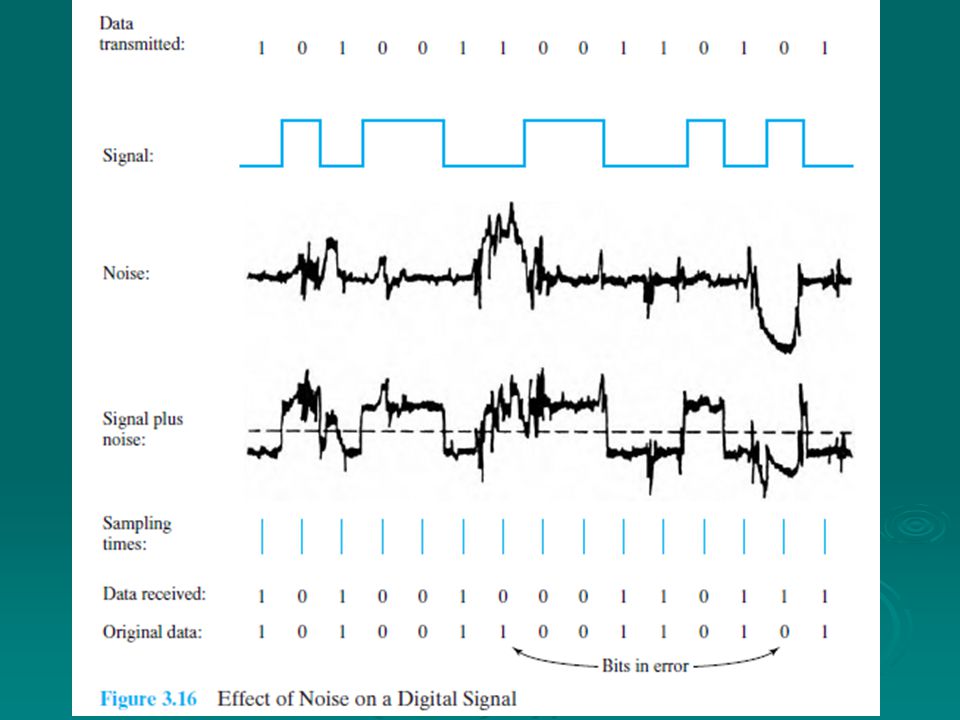
signal received may differ from signal transmitted causing:
analog - degradation of signal quality
digital - bit errors
most significant impairments are
attenuation and attenuation distortion
delay distortion
noise
With any communications system, the signal that is received may differ from the signal that is transmitted due to various transmission impairments. For analog signals, these impairments introduce various random modifications that degrade the signal quality. For digital signals, bit errors may be introduced, such that a binary 1 is transformed into a binary 0 or vice versa. In this section, we examine the various impairments and how they may affect the information-carrying capacity of a communication link; Chapter 5 looks at measures that can be taken to compensate for these impairments.
The most significant impairments are
Attenuation and attenuation distortion
Delay distortion
Noise
Data and Computer Communications, Ninth Edition by William Stallings, (c) Pearson Education - Prentice Hall, 2011

26. Strength can be increased using amplifiers or repeaters.
Received signal strength must be:
strong enough to be detected
sufficiently higher than noise to be received without error
Strength can be increased using amplifiers or repeaters.
Equalize attenuation across the band of frequencies used by using loading coils or amplifiers.
Attenuation
The strength of a signal falls off with distance over any transmission medium. For guided media (e.g., twisted-pair wire, optical fiber), this reduction in strength, or attenuation, is generally exponential and thus is typically expressed as a constant number of decibels per unit distance. For unguided media (wireless transmission), attenuation is a more complex function of distance and the makeup of the atmosphere. Attenuation introduces three considerations for the transmission engineer.
1. A received signal must have sufficient strength so that the electronic circuitry in the receiver can detect and interpret the signal.
2. The signal must maintain a level sufficiently higher than noise to be received without error.
3. Attenuation is greater at higher frequencies, and this causes distortion.
The first and second considerations are dealt with by attention to signal strength and the use of amplifiers or repeaters. For a point-to-point link, the signal strength of the transmitter must be strong enough to be received intelligibly, but not so strong as to overload the circuitry of the transmitter or receiver, which would cause distortion. Beyond a certain distance, the attenuation becomes unacceptably great, and repeaters or amplifiers are used to boost the signal at regular intervals. These problems are more complex for multipoint lines where the distance from transmitter to receiver is variable.
The third consideration, known as attenuation distortion, is particularly noticeable for analog signals. Because attenuation is different for different frequencies, and the signal is made up of a number of components at different frequencies, the received signal is not only reduced in strength but is also distorted. To overcome this problem, techniques are available for equalizing attenuation across a band of frequencies. This is commonly done for voice-grade telephone lines by using loading coils that change the electrical properties of the line; the result is to smooth out attenuation effects. Another approach is to use amplifiers that amplify high frequencies more than lower frequencies.
ATTENUATION
signal strength falls off with distance over any transmission medium
varies with frequency
Data and Computer Communications, Ninth Edition by William Stallings, (c) Pearson Education - Prentice Hall, 2011

27. Noise unwanted signals inserted between transmitter and receiver
is the major limiting factor in communications system performance
Noise
For any data transmission event, the received signal will consist of the transmitted signal, modified by the various distortions imposed by the transmission system, plus additional unwanted signals that are inserted somewhere between transmission and reception. The latter, undesired signals are referred to as noise. Noise is the major limiting factor in communications system performance.
Noise may be divided into four categories:
Thermal noise
Intermodulation noise
Crosstalk
Impulse noise
Data and Computer Communications, Ninth Edition by William Stallings, (c) Pearson Education - Prentice Hall, 2011

28. Thermal noise - White noise
Thermal noise is due to thermal agitation of electrons. It is present in all electronic devices and transmission media and is a function of temperature.
Thermal noise is uniformly distributed across the bandwidths typically used in communications systems and hence is often referred to as white noise.
Thermal noise cannot be eliminated and therefore places an upper bound on communications system performance.

29. intermodulation noise
When signals at different frequencies share the same transmission medium, the result may be intermodulation noise.
The effect of intermodulation noise is to produce signals at a frequency that is the sum or difference of the two original frequencies or multiples of those frequencies.

30. Intermodulation noise
Categories of Noise
Thermal noise
due to thermal agitation of electrons
uniformly distributed across bandwidths
referred to as white noise
Intermodulation noise
produced by nonlinearities in the transmitter, receiver, and/or intervening transmission medium
effect is to produce signals at a frequency that is the sum or difference of the two original frequencies
Thermal noise is due to thermal agitation of electrons. It is present in all electronic devices and transmission media and is a function of temperature. Thermal noise is uniformly distributed across the bandwidths typically used in communications systems and hence is often referred to as white noise. Thermal noise cannot be eliminated and therefore places an upper bound on communications system performance. Because of the weakness of the signal received by satellite earth stations, thermal noise is particularly significant for satellite communication.
The amount of thermal noise to be found in a bandwidth of 1 Hz in any device or conductor is
N0 = kT (W/Hz)
where
N0 = noise power density in watts per 1 Hz of bandwidth
k = Boltzmann's constant = 1.38 ´ 10–23 J/K
T = temperature, in kelvins (absolute temperature), where the symbol K is used to represent 1 kelvin
Example 3.3 Room temperature is usually specified as T = 17˚C, or 290 K. At this temperature, the thermal noise power density is
N0 = (1.38 ´ 10-23) ´ 290 = 4 ´ 10–21 W/Hz = –204 dBW/Hz
where dBW is the decibel-watt, defined in Appendix 3A.
The noise is assumed to be independent of frequency. Thus the thermal noise in watts present in a bandwidth of B hertz can be expressed as
N = kTB
or, in decibel-watts,
N = 10 log k + 10 log T + 10 log B
= –228.6 dBW + 10 log T + 10 log B
Example 3.4 Given a receiver with an effective noise temperature of 294 K and a 10-MHz bandwidth, the thermal noise level at the receiver's output is
N = –228.6 dBW + 10 log(294) + 10 log 107
= –
= –133.9 dBW
When signals at different frequencies share the same transmission medium, the result may be intermodulation noise. The effect of intermodulation noise is to produce signals at a frequency that is the sum or difference of the two original frequencies or multiples of those frequencies. For example, if two signals, one at 4000 Hz and one at 8000 Hz, share the same transmission facility, they might produce energy at 12,000 Hz. This noise could interfere with an intended signal at 12,000 Hz.
Intermodulation noise is produced by nonlinearities in the transmitter, receiver, and/or intervening transmission medium. Ideally, these components behave as linear systems; that is, the output is equal to the input times a constant. However, in any real system, the output is a more complex function of the input. Excessive nonlinearity can be caused by component malfunction or overload from excessive signal strength. It is under these circumstances that the sum and difference frequency terms occur.
Data and Computer Communications, Ninth Edition by William Stallings, (c) Pearson Education - Prentice Hall, 2011

31. Categories of Noise Crosstalk: Impulse Noise:
a signal from one line is picked up by another
can occur by electrical coupling between nearby twisted pairs or when microwave antennas pick up unwanted signals
Impulse Noise:
caused by external electromagnetic interferences
noncontinuous, consisting of irregular pulses or spikes
short duration and high amplitude
minor annoyance for analog signals but a major source of error in digital data
Crosstalk has been experienced by anyone who, while using the telephone, has been able to hear another conversation; it is an unwanted coupling between signal paths. It can occur by electrical coupling between nearby twisted pairs or, rarely, coax cable lines carrying multiple signals. Crosstalk can also occur when microwave antennas pick up unwanted signals; although highly directional antennas are used, microwave energy does spread during propagation. Typically, crosstalk is of the same order of magnitude as, or less than, thermal noise.
All of the types of noise discussed so far have reasonably predictable and relatively constant magnitudes. Thus it is possible to engineer a transmission system to cope with them. Impulse noise, however, is noncontinuous, consisting of irregular pulses or noise spikes of short duration and of relatively high amplitude. It is generated from a variety of causes, including external electromagnetic disturbances, such as lightning, and faults and flaws in the communications system.
Impulse noise is generally only a minor annoyance for analog data. For example, voice transmission may be corrupted by short clicks and crackles with no loss of intelligibility. However, impulse noise is the primary source of error in digital data communication. For example, a sharp spike of energy of 0.01 s duration would not destroy any voice data but would wash out about 560 bits of digital data being transmitted at 56 kbps
Data and Computer Communications, Ninth Edition by William Stallings, (c) Pearson Education - Prentice Hall, 2011

33. Channel Capacity
Maximum rate at which data can be transmitted over a given communications channel under given conditions
data rate
in bits per second
bandwidth
in cycles per second or Hertz
noise
average noise level over path
error rate
rate of corrupted bits
limitations due to physical properties
main constraint on achieving efficiency is noise
We have seen that there are a variety of impairments that distort or corrupt a signal. For digital data, the question that then arises is to what extent these impairments limit the data rate that can be achieved. The maximum rate at which data can be transmitted over a given communication path, or channel, under given conditions, is referred to as the channel capacity.
There are four concepts here that we are trying to relate to one another.
Data rate: The rate, in bits per second (bps), at which data can be communicated
Bandwidth: The bandwidth of the transmitted signal as constrained by the transmitter and the nature of the transmission medium, expressed in cycles per second, or hertz
Noise: The average level of noise over the communications path
Error rate: The rate at which errors occur, where an error is the reception of a 1 when a 0 was transmitted or the reception of a 0 when a 1 was transmitted
The problem we are addressing is this: Communications facilities are expensive and, in general, the greater the bandwidth of a facility, the greater the cost. Furthermore, all transmission channels of any practical interest are of limited bandwidth. The limitations arise from the physical properties of the transmission medium or from deliberate limitations at the transmitter on the bandwidth to prevent interference from other sources. Accordingly, we would like to make as efficient use as possible of a given bandwidth. For digital data, this means that we would like to get as high a data rate as possible at a particular limit of error rate for a given bandwidth. The main constraint on achieving this efficiency is noise.
Data and Computer Communications, Ninth Edition by William Stallings, (c) Pearson Education - Prentice Hall, 2011

34. Summary transmission concepts and terminology
guided/unguided media
frequency, spectrum and bandwidth
analog vs. digital signals
data rate and bandwidth relationship
transmission impairments
attenuation/delay distortion/noise
channel capacity
Nyquist/Shannon
Stallings DCC9e Chapter 3 summary.
Data and Computer Communications, Ninth Edition by William Stallings, (c) Pearson Education - Prentice Hall, 2011