1. Neutrino-interactions in resonance region Satoshi Nakamura Osaka University Collaborators : H. Kamano (RCNP, Osaka Univ.), T. Sato (Osaka Univ.)

2. Introduction

3. Neutrino-nucleus scattering for -oscillation experiments Neutrino-nucleus interactions  neutrino detectors ( 16 O, 12 C, 36 Ar, … ) Neutrino-nucleus interactions need to be known for neutrino flux measurement e.g., T2K @ J-PARC & SuperK

4. DIS region QE region RES region Next-generation exp.  leptonic CP, mass hierarchy  nucleus scattering needs to be understood more precisely Wide kinematical region with different characteristic  Combination of different expertise is necessary Collaboration at J-PARC Branch of KEK Theory Center http://j-parc-th.kek.jp/html/English/e-index.html T2K Neutrino-nucleus scattering for -oscillation experiments Atmospheric

5. Neutrino interaction data in resonance region   p   -  + p   CH 2   -  0 X, PRD 83 (2011) } PRC 87 (2013) Data to fix nucleon axial current ( g  ) Discrepancy between BNL & ANL data Recent reanalysis (arXiv:1411.4482) flux uncertainty  discrepancy resolved (!?) Final state interaction (FSI) changes charge, momentum, number of  Cross section shape is worse described with FSI MINER A data (arXiv:1406.6415) favor FSI GeV More data are coming  better understanding of neutrino-nucleus interaction

6. Resonance region (single nucleon)  2nd 3rd Multi-channel reaction  2  production is comparable to 1    productions ( case: background of proton decay exp.) (MeV)    X

7. GOAL : Develop  -interaction model in resonance region We develop a Unitary coupled-channels model  (multi-channel) Unitarity is missing  Important 2  production model is missing Problems in previous models ★ Dynamical coupled-channels (DCC) model for    ★  Extension to    l - X ( X=   numerical results Our strategy to overcome the problems… Contents of this talk

8. Dynamical Coupled-Channels model for meson productions

9. , Coupled-channel unitarity is fully taken into account Kamano et al., PRC 88, 035209 (2013) In addition,  W ± N, ZN channels are included perturbatively

10. DCC analysis of meson production data Fully combined analysis of    data and polarization observables (W ≤ 2.1 GeV) ~380 parameters (N* mass, N*  MB couplings, cutoffs) to fit ~ 20,000 data points Kamano, Nakamura, Lee, Sato, PRC 88 (2013)

11. Partial wave amplitudes of  N scattering Kamano, Nakamura, Lee, Sato, PRC 88 (2013) Previous model (fitted to  N   N data only) [PRC76 065201 (2007)] Real partImaginary part Data: SAID  amplitude Constraint on axial current through PCAC

12. Kamano, Nakamura, Lee, Sato, 2012 Vector current (Q 2 =0) for 1  Production is well-tested by data Kamano, Nakamura, Lee, Sato, PRC 88 (2013) γp  π 0 p dσ/dΩ for W < 2.1 GeV

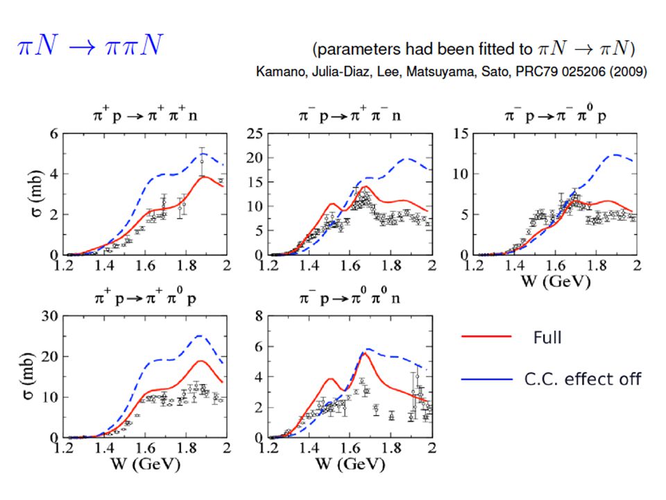
13. Predicted πN  ππN total cross sections with our DCC model Kamano, PRC88(2013)045208 Kamano, Julia-Diaz, Lee, Matsuyama, Sato PRC79(2008)025206 π + p  π + π + nπ - p  π + π - nπ - p  π - π 0 p π + p  π + π 0 pπ - p  π 0 π 0 n

14.  Model for vector & axial currents is necessary Extension to full kinematical region Q 2 ≠0 DCC model for neutrino interaction Forward limit Q 2 =0 Kamano, Nakamura, Lee, Sato, PRD 86 (2012)    X      X  via PCAC

15. Vector current Q 2 =0  p     n      isospin separation necessary for calculating -interaction Q 2 ≠0 (electromagnetic form factors for VNN* couplings) obtainable from ( e,e’  ( e,e’ X  data analysis We’ve done first analysis of all these reactions  VNN*(Q 2 ) fixed  neutrino reactions DCC model for neutrino interaction

16. Q 2 =0 non-resonant mechanisms resonant mechanisms Interference among resonances and background can be made under control within DCC model Axial current DCC model for neutrino interaction Caveat : phenomenological axial currents are added to maintain PCAC relation to be improved in future

17. Axial current Q 2 ≠0 non-resonant mechanisms resonant mechanisms DCC model for neutrino interaction M A =1.02 GeV : axial form factors More neutrino data are necessary to fix axial form factors for ANN * Sato et al. PRC 67 (2003) Neutrino cross sections will be predicted with this axial current for this presentation

18. Analysis of electron scattering data

19. p ( e,e’    p p ( e,e’    n both Analysis of electron-proton scattering data Purpose : Determine Q 2 –dependence of vector coupling of p-N* : VpN*(Q 2 ) Data : * 1  electroproduction Database * Empirical inclusive inelastic structure functions    L  Christy et al, PRC 81 (2010) region where inclusive   &  L are fitted

20. Analysis result Q 2 =0.40 (GeV/c) 2    L for W= 1.1 – 1.68 GeV p ( e,e’    pp ( e,e’    n

21. Analysis result Q 2 =0.40 (GeV/c) 2    L (inclusive inelastic) DCC Christy et al PRC 81  LL region where inclusive   &  L are fitted

22. For application to neutrino interactions Analysis of electron scattering data  VpN*(Q 2 ) & VnN*(Q 2 ) fixed for several Q 2 values  Parameterize VpN*(Q 2 ) & VnN*(Q 2 ) with simple analytic function of Q 2 I=3/2 : VpN*(Q 2 ) =  VnN*(Q 2 )   CC, NC I=1/2 isovector part : ( VpN*(Q 2 )  VnN*(Q 2 ) ) / 2  CC, NC I=1/2 isoscalar part : ( VpN*(Q 2 )  VnN*(Q 2 ) ) / 2  NC DCC vector currents has been tested by data for whole kinematical region relevant to neutrino interactions of E   2 GeV

23. Neutrino Results

24. Caveat Results presented here are still preliminary Careful examination needs to be made to obtain a final result

25. Cross section for   N   - X  are main channels in few-GeV region  Y cross sections are 10 -1 – 10 -2 smaller   n   - X   p   - X

26. Comparison with   N   -  data ANL Data : PRD 19, 2521 (1979) BNL Data : PRD 34, 2554 (1986) DCC model prediction is consistent with data DCC model has flexibility to fit data ( ANN*(Q 2 ) ) Data should be analyzed with nuclear effects   n   -    p   p   -  + p   n   -    n

27. Mechanisms for   N   -   dominates for   p   -    p (I=3/2) for E  GeV Non-resonant mechanisms contribute significantly Higher N * s becomes important towards E  GeV for   n   -    n   -  N   p   -  + p 

28.   n   -  N   n   -  N   p   -  + p   p   -  N E  GeV d  dW dQ 2 ( ×10 -38 cm 2 / GeV 2 )

29. Conclusion

30. Development of DCC model for  interaction in resonance region  are main channels in few-GeV region DCC model prediction for 1  production is consistent with data  N * s, non-resonant are all important in few-GeV region (for   n   - X )  essential to understand interference pattern among them  DCC model can do this; consistency between  interaction and axial current Start with DCC model for     extension of vector current to Q 2 ≠0 region, isospin separation through analysis of e — - p & e — -’n’ data for W ≤ 2 GeV, Q 2 ≤ 3 (GeV/c) 2  Development of axial current for  interaction; PCAC is maintained Conclusion

31. Future development Axial form factor more neutrino data is ideal    ( t -ch  ) (maybe possible at J-PARC)  channel    experiment  (J-PARC, K. Hicks et al.)    experiment  (ELPH, JLab) Nuclear models deuteron model,  -hole type model

32. BACKUP

33. Contents ★ Introduction  scattering in resonance region ★ Dynamical coupled-channels (DCC) model  Analysis of      data  Extension to    l - X ( X=  ★ Results for    l - X

34. Physics at J-PARC: Charm, Neutrino, Strangeness, and Spin T2K (Tokai to Kamioka) experiment for neutrino oscillation measurement Far Detector (Super Kamiokande) T2K measures neutrino fluxes at near and far detectors J-PARC produces neutrino beam directed to Super Kamiokande by Proton + nucleus    (   ) + ….           _

35. Neutrino oscillation Expected  fluxes in T2K Near detector Far detector E  (GeV)  survival probability (two-flavor case)  mixing angle  m 2 (eV 2 ) = m  2 – m  2 L (km) : distance between J-PARC and SK   (GeV) : neutrino energy Comparing data to oscillation formula, mixing parameters (  m 2 ) can be determined Comparing data with  data  leptonic CP violation (  CP ) _

36. T2K Quasi-elastic (QE) is dominant -flux is measured by detecting QE 1  production via  excitation is major background  can be absorbed  QE is contaminated      LBNE and other planned experiments ( higher energy -beam) DIS and higher nucleon resonances are main mechanisms In this work, we focus on resonance region, single nucleon processes  basic ingredient for neutrino-nucleus interaction model

37. DCC model for neutrino interaction    X  is from our DCC model via PCAC   l X ( X =  ) at forward limit Q 2 =0 Kamano, Nakamura, Lee, Sato, PRD 86 (2012) NN  N 

38. Formalism Cross section for   l X ( X =  )    Q2Q2 CVC & PCAC LSZ & smoothness Finally    X  is from our DCC model

39. Results SL NN  N  NN   Prediction based on model well tested by data (first      dominates for W ≤ 1.5 GeV   becomes comparable to  for W ≥ 1.5 GeV  Smaller contribution from  and  Y O (10 -1 ) - O (10 -2 )  Agreement with SL (no PCAC) in  region

40. Comparison with Rein-Sehgal model Lower  peak of RS model  RS overestimate in higher energy regions (DCC model is tested by data) Similar findings by Leitner et al., PoS NUFACT08 (2008) 009 Graczyk et al., Phys.Rev. D77 (2008) 053001 Comparison in whole kinematical region will be done after axial current model is developed

41. F 2 from RS model

42. SL model applied to  nucleus scattering 1  production Szczerbinska et al. (2007)

43. SL model applied to  nucleus scattering coherent  production   C       C    C    - +     C Nakamura et al. (2010)

45. Previous models for induced 1  production in resonance region Rein et al. (1981), (1987) ; Lalalulich et al. (2005), (2006) Hernandez et al. (2007), (2010) ; Lalakulich et al. (2010) Sato, Lee (2003), (2005) resonant only + non-resonant (tree-level) + rescattering (  N unitarity)

46. Eta production reactions Kamano, Nakamura, Lee, Sato, 2012

47. KY production reactions 1732 MeV 1845 MeV 1985 MeV 2031 MeV 1757 MeV 1879 MeV 1966 MeV 2059 MeV 1792 MeV 1879 MeV 1966 MeV 2059 MeV Kamano, Nakamura, Lee, Sato, 2012

49. Kamano, Nakamura, Lee, Sato, arXiv:1305.4351 Vector current (Q 2 =0) for  Production is well-tested by data

50. Vector current (Q 2 =0) for  Production is well-tested by data Kamano, Nakamura, Lee, Sato, arXiv:1305.4351

52. Kamano, Nakamura, Lee, Sato, PRC 88 (2013) “N” resonances (I=1/2) J P (L 2I 2J ) Re(M R ) “Δ” resonances (I=3/2) PDG: 4* & 3* states assigned by PDG2012 AO : ANL-Osaka J : Juelich (DCC) [EPJA49(2013)44, Model A] BG : Bonn-Gatchina (K-matrix) [EPJA48(2012)5] -2Im(M R ) (“width”)

53. Kamano, Nakamura, Lee, Sato, 2012 Quality of describing data with DCC model Model is extensively tested by    data ( W ≤ 2.1 GeV, ~ 20,000 data points)  application to -scattering reliable vector current ( Q 2 = 0)   X model combined with PCAC Kamano, Nakamura, Lee, Sato, PRC 88 (2013)

54. Analysis result Q 2 =0.16 (GeV/c) 2    L for W= 1.1 - 1.32 GeV p ( e,e’    pp ( e,e’    n

55. Analysis result Q 2 =0.16 (GeV/c) 2    L (inclusive inelastic) DCC Christy et al PRC 81  LL region where inclusive   &  L are fitted

56. Analysis result Q 2 =2.95 (GeV/c) 2    L for W= 1.11 – 1.69 GeV p ( e,e’    pp ( e,e’    n

57. Analysis result Q 2 =2.95 (GeV/c) 2    L (inclusive inelastic) DCC Christy et al PRC 81  LL region where inclusive   &  L are fitted

58. Purpose : Vector coupling of neutron-N * and its Q 2 –dependence : VnN*(Q 2 ) (I=1/2) I=3/2 part has been fixed by proton target data Analysis of electron-’neutron’ scattering data Data : * 1  photoproduction ( Q 2 =0) * Empirical inclusive inelastic structure functions    L ( Q 2 ≠ 0)  Christy and Bosted, PRC 77 (2010), 81 (2010)

59. Analysis result Q 2 =0 d    d  (  n    p) for W= 1.1 – 2.0 GeV

60. Analysis result Q 2 =1 (GeV/c) 2    L (inclusive inelastic e — -’n’ ) DCC Christy and Bosted PRC 77; 81  LL Q 2 =2 (GeV/c) 2 LL  Q 2 ≠0