1. Chapter 13 The Rates of Reactions St. John’s wort （貫葉連翹 / 金絲 桃 / 聖約翰草） is an herb that is thought to create a sense of tranquility. Herbs and other medicines have been used through the ages to cure disease and to relieve pain. In many cases, the medicine is effective because it controls the rates of reactions within the body. In this chapter, we examine the rates of chemical reactions and the mechanisms by which they take place.

2. Assignment for Chapter 13 13.22; 13.31; 13.37; 13.61

6. How to Live Longer and More Healthy? Reduction of food Cold body temperature Appropriate exercise Good temper Demonstrated tips: All related to (slower) chemical reaction rates.

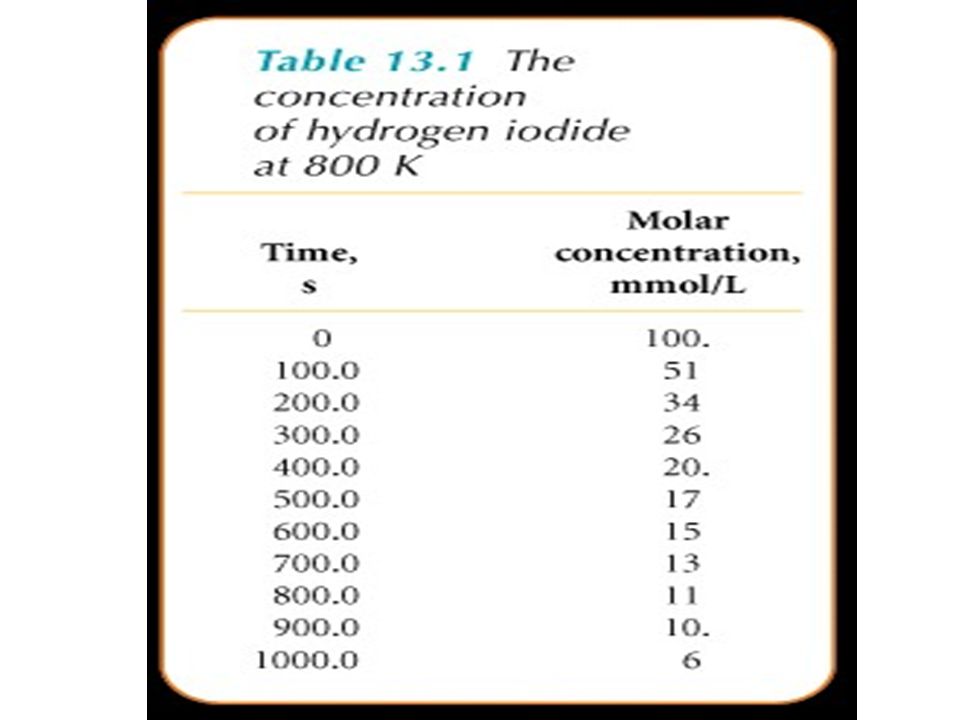
7. Definition kA  mC+nD Rate=change in concentration of reactant / time interval 2HI(g)  H 2 (g)+I 2 (g)

11. Figure 13.1 The activity of penicillin declines over several weeks when it is stored at room temperature in the absence of stabilizers. The shape of this graph of concentration of penicillin as a function of time is typical of the behavior of chemical reactions, although the time span may vary from fractions of a second to years.

12. Figure 13.2 This graph shows two examples of how the rate of consumption of penicillin can be monitored while it is being stored. The red line shows the average rate calculated from measurements at 0 and 10 weeks, and the blue line shows the average rate calculated from measurements at 2.5 and 7.5 weeks. The instantaneous rate at 5 weeks is the tangent to the curve at that time (not shown).

13. Figure 13.3 To calculate the instantaneous reaction rate, we draw the tangent to the curve at the time of interest and then calculate the slope of this tangent. To calculate the slope, we identify any two points, A and B, on the straight line and identify the molar concentrations and times to which they correspond. The slope is then worked out by dividing the difference in concentrations by the difference in times. Notice that this graph shows the concentration of a product.

14. Figure 13.4 The initial rate of reaction for the decomposition of N 2 O 5 in five experiments. The initial rate of disappearance of a reactant is determined by drawing a tangent to the curve at the start of the reaction. 2N 2 O 5 (g)  4NO 2 (g)+O 2 (g)

15. Figure 13.5 The plot of the initial rate of decomposition of N 2 O 5 as a function of initial concentration for the five samples in Fig. 13.4 is a straight line. The linear plot shows that the rate is proportional to the concentration. The graph also illustrates how we calculate the rate constant, k, from the slope of the straight line.

16. Initial rate=k × initial concentration

17. Figure 13.6 (a) The instantaneous reaction rates for the decomposition of N 2 O 5 at five different times during a single experiment are obtained from the slopes of the tangents to the line at each of the five points. (b) When these rates (the slopes) are plotted as a function of the concentration of N 2 O 5 remaining, the result is a straight line with a slope equal to the rate constant. In (b), we have indicated the rates by redrawing the tangents.

18. a: order of reaction, determined by experiment.

19. Figure 13.7 (a) The concentration of the reactant in a zero- order reaction falls at a constant rate until the reactant is exhausted. (b) The rate of a zero-order reaction is independent of the concentration of the reactant and remains constant until all the reactant has been consumed, when it falls abruptly to 0.

20. There are no images in this section of the chapter. More General Cases:... ][][   baorderOverall BAkR b a 2 3 ][ 22 3 ]][ [ )(3)(3 )(6)(5)( 3         H Br BrOk lOHaqBr aqH BraqBrO t

22. Example Initial concentration, mol/L ExperimentBrO 3 - Br - H+ Initial rate (mol BrO 3 - )/L/sec 10.10 1.2×10 -3 20.200.10 2.4×10 -3 30.100.30 0.103.5×10 -3 40.200.10 0.155.4×10 -3 Find the rate law for the disappearance of bromate ions in the reaction: With respect to each reactant and determine k given the following data

23. Example Initial concentration, mol/L ExperimentBrO 3 - Br - H+ Initial rate (mol BrO 3 - )/L/sec 10.10 1.2×10 -3 20.200.10 2.4×10 -3 30.100.30 0.103.5×10 -3 40.200.10 0.155.4×10 -3

24. More Complicated Rate Laws Order=a+b+…-p-…

25. Figure 13.8 (a) When sulfur dioxide and oxygen are passed over hot platinum foil, they combine to form sulfur trioxide. (b) The sulfur trioxide forms dense white fumes of sulfuric acid when it comes into contact with moisture in the atmosphere. The rate law for the formation of sulfur trioxide shows that its rate of formation decreases as its concentration increases, so the sulfur trioxide must be removed as it is formed if the reaction is to proceed rapidly. 2SO 2 (g)+O 2 (g)  2SO 3 (g)

26. Classroom Exercise Initial concentration, mol/L ExperimentS 2 O 8 2- I-I- Initial rate (mol S 2 O 8 2- )/L/sec 10.150.211.14 20.220.211.70 30.220.120.98 Find the rate law for the disappearance of persulfate ions in the reaction: With respect to each reactant and determine k given the following data

27. Classroom Exercise Initial concentration, mol/L ExperimentS 2 O 8 2- I-I- Initial rate (mol S 2 O 8 2- )/L/sec 10.150.211.14 20.220.211.70 30.220.120.98

28. Integrated Rate Law Find the concentration of a reactant at time t from reaction order and initial concentration. First order reaction:

29. Figure 13.9 The characteristic shape of the graph showing the time dependence of the concentration of a reactant in a first- order reaction is an exponential decay, as shown here. The larger the rate constant, the faster the decay from the same initial concentration.

30. Example 2N 2 O 5 (g)  4NO 2 (g)+O 2 (g) (65 o C) Rate =k[N 2 O 5 ], k=5.2×10 -3 /s Initial concentration of N 2 O 5 was 0.04 mol/L. What is its concentration after 10 minutes?

31. How to find k (first order reaction):

32. Example Time, min Concentration of cyclopropane, mol/L 0 5.0 10.0 15.0 1.5×10 -3 1.24×10 -3 1.00×10 -3 0.83×10 -3

33. Example Time, min ln[cyclopropane] 0 5.0 10.0 15.0 -6.5 -6.69 -6.91 -7.09

34. Figure 13.10 We test for a first-order reaction by plotting the natural logarithm of the reactant concentration as a function of time. The slope of the line, which is calculated as indicated in the illustration by selecting two points A and B, is equal to the negative of the rate constant. Time, min ln[cyclopropane] 0 5.0 10.0 15.0 -6.5 -6.69 -6.91 -7.09

35. Classroom Exercise Time, min Concentration of N 2 O 5, mol/L 0 200.0 400.0 600.0 800.0 1000.0 1.5×10 -2 9.6×10 -3 6.2×10 -3 4.0×10 -3 2.5×10 -3 1.6×10 -3 2N 2 O 5 (g)  4NO 2 (g)+O 2 (g) (25 o C) Find the rate constant k at this temperature.

36. Classroom Exercise Time, min ln [N 2 O 5 ] 0 200.0 400.0 600.0 800.0 1000.0 ln(1.5×10 -2 )=-6.5022 ln(9.6×10 -3 )=-6.9485 ln(6.2×10 -3 )=-7.3858 ln(4.0×10 -3 )=-7.8240 ln(2.5×10 -3 )=-8.2940 ln(1.6×10 -3 )=-8.7403 Slope = - 2.2×10 -3 /min k=2.2×10 -3 /min Time (min) ln[N2O5] 200 400 600 800 1000 -6.5 -7.5 -8.0 -7.0 -8.5 -9.0

37. Half-Lives of First Order Reactions

38. Figure 13.11 The half-life of a reactant is short if the first-order rate constant is large, because the exponential decay of the concentration of the reactant is then faster.

39. Figure 13.12 The half-life of a substance is the time needed for it to fall to one-half its initial concentration. For first-order reactions, the half-life is the same whatever the concentration at the start of the chosen period. Therefore, it takes one half-life for the concentration to fall to half the initial value, two half-lives for the concentration to fall to one-fourth the initial value, three half-lives to fall to one-eighth, and so on.

40. Example A pollutant escapes into a local picnic site. Studies show that the pollutant decays by a first order reaction with rate constant 3.8×10 -3 /h. Calculate the time needed for the concentration to fall to (a) one half and (b) one-fourth of its initial value.

41. Classroom Exercise A pollutant escapes into a local picnic site. Studies show that the pollutant decays by a first order reaction with rate constant 3.8×10 -3 /h. Calculate the time needed for the concentration to fall to one-eigth of its initial value.

42. Second Order Integrated Rate Laws 2A  A+A

43. Figure 13.13 The characteristic shapes (orange and green lines) of the time dependence of the concentration of a reactant during two second-order reactions. The gray lines are the curves for first-order reactions with the same initial rates. Note how the concentrations for second-order reactions fall away much less rapidly than those for first-order reactions do.

44. Figure 13.14 A summary of the plots that give straight lines for first- and second-order reactions.

45. Controlling Reaction Rates Surface Area Temperature Pressure Catalyst Activated Complex Theory

46. Figure 13.15 A solid iron rod can be heated in a flame without catching fire. However, a powder of very finely divided iron oxidizes rapidly in air to form Fe 2 O 3, because the powder presents a much greater surface area for reaction with oxygen.

47. Figure 13.16 The Hindenburg, a hydrogen-filled airship, caught fire as it came in to land at Lakehurst, New Jersey in 1937 after its inaugural flight across the Atlantic. The hydrogen was ignited when the airship collided with an electrical tower.

48. Temperature Dependence of Reaction Rates 2N 2 O 5 (g)  4NO 2 (g)+O 2 (g) (25 o C) 2N 2 O 5 (g)  4NO 2 (g)+O 2 (g) (65 o C) k=5.2×10 -3 /s k=2.2×10 -3 /s Preexponent factor Activation energy

49. Figure 13.17 An Arrhenius plot is a graph of ln k against 1/T. If, as here, the line is straight, then the reaction is said to show Arrhenius behavior in the temperature range studied. The activation energy for the reaction is obtained by setting the slope of the line equal to  E a /R. SvanteA Arrhenius (1859-1927)

50. Measuring Activation Energy C 2 H 5 Br(aq)+OH - (aq)  C 2 H 5 OH(aq)+Br - (aq) Temperature ( o C) k (L/mol/s) 258.8×10 -5 301.6×10 -4 352.8×10 -4 405.0×10 -4 458.5×10 -4 501.4×10 -3 Find Ea.

51. Measuring Activation Energy Temperature ( o C) T 1/T k (L/mol/s) lnk 25 298 3.35 ×10 -3 8.8×10 -5 -9.34 30 303 3.30 ×10 -3 1.6×10 -4 -8.74 35 308 3.25 ×10 -3 2.8×10 -4 -8.18 40 313 3.19 ×10 -3 5.0×10 -4 -7.60 45 318 3.14 ×10 -3 8.5×10 -4 -7.07 50 323 3.10 ×10 -3 1.4×10 -3 -6.57

52. Figure 13.18 An Arrhenius plot of the data in Example 13.7. The slope of the line has been worked out by using points A and B. Temperature ( o C) T 1/T k (L/mol/s) lnk 25 298 3.35 ×10 -3 8.8×10 -5 -9.34 30 303 3.30 ×10 -3 1.6×10 -4 -8.74 35 308 3.25 ×10 -3 2.8×10 -4 -8.18 40 313 3.19 ×10 -3 5.0×10 -4 -7.60 45 318 3.14 ×10 -3 8.5×10 -4 -7.07 50 323 3.10 ×10 -3 1.4×10 -3 -6.57

54. Classroom Exercise OH (g)+H 2 (g)  H 2 O (g)+H (g) Temperature ( o C) k (L/mol/s) 1001.1×10 -9 2001.8×10 -8 3001.2×10 -7 4004.4×10 -7 Find Ea.

55. Temperature ( o C) T 1/T k (L/mol/s) lnk 100 373 2.51 ×10 -3 1.1×10 -9 -19.63 200 473 2.01×10 -3 1.8×10 -8 -17.83 300 573 1.67 ×10 -3 1.2×10 -7 -15.94 400 673 1.43 ×10 -3 4.4×10 -7 -14.64 Classroom Exercise 1/T (K -1 ) ×10 3 lnk 1.0 1.5 2.0 2.5 3.0 -10 -14 -16 -12 -18 -20

56. Figure 13.19 The variation of the rate constant with temperature for different values of the activation energy. Note that the higher the activation energy, the more strongly the rate constant varies with temperature.

57. Example The rate constant of sucrose hydrolysis (sucrose is broken down into glucose and fructose) at body temperature is 1.0×10 -3 L/mol/s. The activation energy of the reaction is 108 kJ/mol. What would it be at 35 o C?

58. Classroom Exercise The rate constant of the first order isomerization of cyclopropane to propene is 6.7×10 -4 /s at 500 o C. The activation energy of the reaction is 272 kJ/mol. What would it be at 300 o C?

59. Figure 13.20 (a) In the collision theory of chemical reactions, reaction can occur only when two molecules collide with a kinetic energy at least equal to the activation energy of the reaction. (b) Otherwise they simply bounce apart.

60. Figure 13.21 A reaction profile for an exothermic reaction. In the collision theory of reaction rates, the potential energy (the energy due to position) increases as the reactant molecules approach each other, reaches a maximum as the molecules distort, and then decreases as the atoms rearrange into the bonding pattern characteristic of the products and these products separate. Only molecules with sufficient energy can cross the barrier and react to form products.

61. Figure 13.22 The fraction of molecules that collide with a kinetic energy that is at least equal to the activation energy, E a, is denoted by the shaded areas under each curve. The fraction increases rapidly as the temperature is raised.

62. Figure 13.23 Whether or not a reaction occurs when two species collide in the gas phase depends on their relative orientation as well as on their energies. In the reaction between a Cl atom and an HI molecule, for example, only those collisions in which the Cl atom approaches the HI molecule along a path that lies inside a cone centered on the H atom lead to reaction, even though the energies of collisions in other orientations may exceed the activation energy.

63. Figure 13.24 This sequence of images illustrates the motion of two reactant molecules (red and green) in solution. The blue spheres represent solvent molecules. We see the reactants drifting together, lingering near each other for some time, and then drifting apart again. Reaction may occur during the relatively long period of encounter. To highlight the positions of the reactant molecules, the insets show the solvent molecules as a solid blue background.

64. Figure 13.25 We join this sequence of images at the moment when the reactant molecules are in the middle of their encounter. They may acquire enough energy by impacts from the solvent molecules to form an activated complex, which may go on to form products. Once again, the insets highlight the reactants by showing the solvent molecules as a solid blue background. Activated Complex Theory Activated Complex

65. Figure 13.26 The reaction profile for the activated complex theory of reactions in solution, in which the reactants form an activated complex, provided they encounter each other with at least the activation energy.

66. Catalysis Catalyst Homogeneous catalysis Heterogeneous catalysis Poisoning of catalyst Enzyme (living catalyst)

67. Figure 13.27 A catalyst provides a new reaction pathway with a lower activation energy, thereby allowing more reactant molecules to cross the barrier and form products. Notice that E a for the reverse reaction is also lowered on the catalyzed path.

68. Figure 13.28 A small amount of catalyst—in this case, potassium iodide in aqueous solution—can accelerate the decomposition of hydrogen peroxide to water and oxygen. This effect is shown (a) by the slow inflation of the balloon when no catalyst is present and (b) by its rapid inflation when a catalyst is present. Homogeneous catalysis

69. Figure 13.29 The reaction between ethene, CH 2  CH 2, and hydrogen on a catalytic metal surface. In this sequence of images, we see the ethene molecule approaching the metal surface to which hydrogen molecules have already adsorbed: when they adsorb, they dissociate and stick to the surface as hydrogen atoms. After sticking to the surface, the ethene molecule meets a hydrogen atom and forms a bond. At this stage (center), a ·CH 2 CH 3 radical is attached to the surface by one of its carbon atoms. Finally, the radical and another hydrogen atom meet, ethane is formed, and the product escapes from the surface. CH 2  CH 2  ·CH 2 CH 3 +H  CH 3 CH 3

70. Figure 13.30 The internal structure of a zeolite is like a honeycomb of passages and cavities. As a result, a zeolite presents a huge surface area. It can also permit the entry and exit of molecules of a certain size into the active regions within the holes. This zeolite is ZSM-5.

71. Figure 13.31 The structure of a typical catalytic converter for an automobile exhaust. The gases flow through a honeycomblike porous ceramic support covered with catalyst.

72. Figure 13.32 The lysozyme （溶菌酶） molecule shown here is a typical enzyme molecule. Lysozyme occurs in a number of places, including tears and the mucus in the nose. One of its functions is to attack the cell walls of bacteria and destroy them. In this illustration the winding ribbon represents the long chain that makes up the molecule.

73. Figure 13.33 In the lock-and-key model of enzyme action, the correct substrate is recognized by its ability to fit into the active site like a key into a lock. In a refinement of this model, the enzyme changes its shape slightly as the key enters.

74. Figure 13.34 (a) An enzyme poison (represented by the mottled green rectangle) can act by attaching so strongly to the active site that it blocks the site, thereby taking the enzyme out of action. (b) Alternatively, the poison molecule may attach elsewhere, so distorting the enzyme molecule and its active site that the substrate no longer fits.

75. Case Study 13 (a) A plot of Michaelis-Menten enzyme kinetics (1913). At low substrate concentrations, the rate of reaction is directly proportional to substrate concentration. However, at high substrate concentrations, the rate is constant, as the enzyme molecules are “saturated” with substrate. Look at the shape of the graph. At low [S], it is the availability of substrate that is the limiting factor. Therefore as more substrate is added there is a rapid increase in the initial rate of the reaction - any substrate is rapidly mopped up and converted to product. At the K M, 50% of active sites have substrate bound. At higher [S] a point is reached (at least theore- tically) where all of the enzyme has substrate bound and is working flat out. Adding more substrate will not increase the rate of the reaction, hence the leveling out observed in the graph. V [S] KMKM V max 0.5V max Leonor Michaelis, Maud Menten 1875-1949 1879–1960

76. Case Study 13 (b) A diagram of a synapse. The triangles represent neurotransmitters that travel from the neuron on the left to the receptors in the neuron on the right. The concentration of neurotransmitters in the synapse is controlled by enzymes.

77. Dopamine OH NH 2 （多巴胺）

78. Case Study 13 (c) The neurons in the human brain affect how we think and feel and how we perceive reality, including chemistry books.

79. Reaction Mechanisms Elementary Reaction Molecularity (Unimolecular, Bimolecular Termolecular Reactions) Reaction Intermediate Rate Law Rate Determining Step (RDS) Chain Reaction

80. Figure 13.35 The chemical equations for elementary reactions show the individual events that take place when atoms and molecules encounter one another. This illustration shows two of the steps believed to occur during the formation of hydrogen iodide from hydrogen and iodine vapor. In one, I 2  I 2  I 2  I  I, a collision between two iodine molecules results in the dissociation of one of them. In the second step, I  H 2  H  HI, one of the I atoms produced in the first step attacks a hydrogen molecule and forms a hydrogen iodide molecule and a hydrogen atom. I 2  I 2  I 2  I  I, I  H 2  H  HI I 2 +H 2  2HI

81. Many reactions occur by a series of elementary reactions. The molecularity of an elementary reaction indicates how many species are involved in that step.

82. The Rate Laws of Elementary Reactions A unimolecular reaction depends on a single energized species shaking itself apart and always has a first order rate law: X  products Rate of disappearance of X =k[X]. A bimolecular reaction depends on collisions between two species, so its rate law is second order: X+X  products Rate of disappearance of X =k[X] 2. X+Y  products Rate of disappearance of X =k[X][Y]. From elementary rate laws to construct overall rate law can be hard, simplifications (e.g., rate determining step) are normally evoked.

83. Rate Determining Step(RDS) The elementary reaction that is much slower than the rest and governs the overall reaction.

84. Figure 13.36 The rate of a reaction is controlled by the rate-determining step (RDS). (a) If the rate-determining step is the second step, then the rate law for that step determines the rate law for the overall reaction. The orange curve shows the reaction profile for such a mechanism, with a high activation energy for the slow step. The concentrations of intermediates can usually be expressed in terms of reactants and products by taking into account the steps preceding the RDS. (b) If the rate-determining step is the first step, then the rate law for that step must match the rate law for the overall reaction. Later steps do not affect the rate or the rate law. (c) If two parallel paths lead to products, the faster one (in this case, the lower one) determines the rate of the reaction.

85. Example

86. From Mechanism to Overall Rate Law

87. Classroom Exercise

88. From Overall Rate Law to Reaction Mechanism

91. Suppose step 1 forward is RDS  Rate law: k 1 [Br 2 ][NO], disagreement with experimental result. Suppose step 2 is RDS  Rate law: k 2 [NOBr 2 ][NO], again, disagreement with experimental result.

92. From Overall Rate Law to Reaction Mechanism Suppose step 1 forward and reverse are much faster than step 2. k 1 [Br 2 ][NO] = k 1 ’ [NOBr 2 ] Suppose step 2 is RDS  Rate law: k 2 [NOBr 2 ][NO]= (k 2 k 1 /k 1 ’)[NO] 2 [Br 2 ]

93. Case Study 13 (a) A plot of Michaelis-Menten enzyme kinetics. At low substrate concentrations, the rate of reaction is directly proportional to substrate concentration. However, at high substrate concentrations, the rate is constant, as the enzyme molecules are “saturated” with substrate. V [S] KMKM V max 0.5V max E+S ES E+P RDS

94. V [S] KMKM V max 0.5V max The overall rate of the reaction (v) is limited by the step ES to E + P, and this will depend on two factors - the rate of that step (i.e. k 2 ) and the concentration of enzyme that has substrate bound, i.e. [ES]. This can be written as: The first step is fast and the forward and reverse reactions keep equilibrium: ( where The total amount of enzyme is constant: or Derivation of Michaelis-Menten Equation

95. Figure 13.37 In a chain reaction, the product of one reaction step is a reactant in a subsequent step, which in turn produces species that can take part in subsequent reaction steps. Initiation Propagation

96. Example (I)

97. Figure 13.38 This flame front was caught during the rapid combustion that occurs inside an internal combustion engine every time a spark plug ignites gasoline vapor. This radical chain reaction occurs in automobile engines. The products, which are hot gases, push a piston out, initiating a chain of events that ultimately moves the vehicle.

98. Example (II): Branching Chain Reaction

99. Assignment for Chapter 13 13.22; 13.31; 13.37; 13.61