1. 2011.06.01 Beyond Trilateration: On the Localizability of Wireless Ad Hoc Networks Reported by: 莫斌

2. Authors Zheng Yang Hong Kong University of Science and Technology Yuhao Liu Hong Kong University of Science and Technology Xiang-Yang Li Illinois Institute of Technology

3. Outline INTRODUCTION NEIGHBORHOOD LOCALIZABILITY NETWORK-WIDE LOCALIZABILITY PERFORMANCE EVALUATION CONCLUSION

4. Supplementary Material  What is Trilateration?  Trilateration is proposed for testing localizability based on the fact that the location of an object can be determined if the distances to three references are known.

5. Supplementary Material  What is Rigidity?  Rigidity is the property of a structure that it does not bend or flex under an applied force. The opposite of rigidity is flexibility.

6. Supplementary Material  What is Connectivity of graph theory?  A cut, vertex cut, or separating set of a connected graph G is a set of vertices whose removal renders G disconnected. The connectivity is the size of a smallest vertex cut.  This means a graph G is said to be k-connected if there does not exist a set of k-1 vertices whose removal disconnects the graph.

7. INTRODUCTION  The proliferation of wireless and mobile devices has fostered the demand of context-aware applications.  Location is one of the most essential contexts.

8. INTRODUCTION  Beacons know their global locations and the rest determine their locations by measuring the Euclidean distances to their neighbors.

9. INTRODUCTION  A wireless ad hoc network can be modeled by a distance graph G=(V, E, d).  A graph with possible additional constraint is called localizable if there is a unique location of every node.

10. INTRODUCTION  A graph is called rigid if one cannot continuously deform the graph embedding in the plane while preserving the distance constraints.  A graph is redundantly rigid if the removal of any edge results in a graph that is still rigid.

11. INTRODUCTION  A graph is globally rigid if there is a unique realization in the plane.  Jackson et al. prove that a graph is globally rigid if and only if it is 3-connected and redundantly rigid.

12. INTRODUCTION  Global information is needed to test connectivity.

13. INTRODUCTION  Trilatertion-based approaches.  Border nodes are often more critical in many applications.

14. INTRODUCTION  A algorithm to find localizable nodes by testing whether they are included in some wheel graphs within their neighborhoods.  Using only local information, it is able to recognize all one-hop localizable nodes.

15. NEIGHBORHOOD LOCALIZABILITY  Lemma 1: The wheel graph W n is globally rigid.  Proof: The graph Wn is redundantly rigid and 3-connected. Accordingly, it is globally rigid.

16.  Conditions for Node Localizability  N[v] is a subgraph of G n containing only v and its one-hop (direct) neighbors and edges between them in G n.  N(v) is obtained by removing v and all edges incident to v from N[v]. NEIGHBORHOOD LOCALIZABILITY

17.  if a vertex in N[v] is included in a wheel graph centered at v, it is localizable by given three beacons.  three localizable vertices in N[v].  the hub and two rim vertices;  three rim vertices. NEIGHBORHOOD LOCALIZABILITY

18.  Vertex x belongs to a wheel structure in N[v] including two localizable vertices v 1 and v 2.  X lies on a cycle containing v 1 and v 2 in N(v). NEIGHBORHOOD LOCALIZABILITY

19.  According to Dirac’s result, if a graph G is 3-connected, for any three vertices in G, G has a cycle including them.  If N(v) is 3-connected, all vertices are included in some wheels in N[v]. NEIGHBORHOOD LOCALIZABILITY It’s too critical to be realistic.

20.  As we know, a 2-connected component in a graph G is a maximal subgraph of G without any articulation vertex whose removal will disconnect G.  For simplicity, we use blocks to denote 2- connected components. NEIGHBORHOOD LOCALIZABILITY

21.  Lemma 2: In a graph G with an edge (v 1,v 2 ), a vertex x belongs to the block B including v 1 and v 2 if and only if it is on a cycle containing v 1 and v 2.  Sufficiency. B’ Is a block, and there are at least two vertex- disjoint paths between any two vertices.  Necessity. contradicting the maximality assumption of blocks.

22. NEIGHBORHOOD LOCALIZABILITY  Lemma 3: If a graph G is 2-connected, then G’ is globally rigid, where G’ is obtained by adding a vertex v 0 and edges between v 0 to all vertices in G.  We take an arbitrary edge (v 1,v 2 ) in G. every other vertex x in G is on a cycle containing v 1 and v 2 by Lemma 2.  Since every wheel in G’ shares three vertices, all vertices are actually in the only one globally rigid component.

23.  Note that not all blocks in N(v) are localizable. NEIGHBORHOOD LOCALIZABILITY

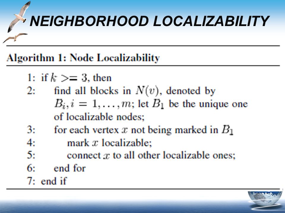
24.  Theorem 1: In a neighborhood graph N[v] with k (k>=3) localizable vertices v i (i=1,…,k and v= v k ), a vertex (other than v i ) belongs to a wheel structure with at least three localizable vertices if and only if it is included in the only (unique) block of N(v) that contains k-1 localizable vertices.  Sufficiency: According to Lemma 2.  Necessity: According to Lemma 2 and by adding v k back.

25.  So far, we achieve a necessary and sufficient condition for finding localizable vertices.  Trilateration is actually the minimum wheel graph with four vertices. NEIGHBORHOOD LOCALIZABILITY

27.  Is there any localizable vertex that is not included by any wheel in N[v]?  Lemma 4: In a graph G, if a vertex is uniquely localizable, it must have three vertex-disjoint paths to three distinct localizable vertices.  Theorem 2: (Correctness) In a neighborhood graph N[v], a vertex is marked by Algorithm 1 if and only if it is uniquely localizable in N[v]. NEIGHBORHOOD LOCALIZABILITY

28.  Proof for Theorem 2:  Sufficiency: Algorithm 1 finds wheel structures with at least three beacons in N[v]. According to Lemma 1.  Necessity: According to Lemma 4. NEIGHBORHOOD LOCALIZABILITY

29.  Definition 1: A graph G is a wheel extension if there are the following:  three pairwise-connected vertices, say v 1, v 2 and v 3 ;  an ordering of remaining vertices as v 4, v 5, v 6 …, such that any v i is included in a wheel graph (a subgraph of G) containing three early vertices in the sequence. NETWORK-WIDE LOCALIZABILITY  Lemma 5: The wheel extension is globally rigid.  The proof of Lemma 5 is straightforward.

30. NETWORK-WIDE LOCALIZABILITY

31.  Analyze the time complexity of Algorithm 2 running on a graph G with n vertices.  O(n 3 ) in dense graphs and O(n) in sparse graphs.  In practice, a wireless ad hoc network cannot be excessively dense because the communication links only exist between nearby nodes due to signal attenuation. NETWORK-WIDE LOCALIZABILITY

32.  The localizability protocol is implemented on the hardware platform of the OceanSense project.  We equip five out of 60 nodes with GPS receivers and adopt the RSS-based ranging technique.  We collect a number of instances of the network topology from 8-h observation.  Trilateration (TRI) is chosen as a representative of all trilateration-based approaches. PERFORMANCE EVALUATION

34.  Large-scale simulations are further conducted to examine the effectiveness and scalability of this design.  We generate networks of 400 nodes randomly, uniformly deployed in a unit square [0,1] 2.  The unit disk model with a radius is adopted for communication and distance ranging.  For each evaluation, we integrate results from 100 network instances. PERFORMANCE EVALUATION

37. r=0.15

38. r=0.16

39. CONCLUSION  Analyze the limitation of trilateration-based approaches.  Propose a novel approach, called WHEEL, based on globally rigid wheel graphs.  To validate this approach, a prototype system with tens of wireless sensors is deployed.  Large-scale simulations are further conducted to evaluate the scalability and efficiency.

41.  Definition 2: In a network, a node is k-hop localizable if it can be localized by using only the information of at most k-hop neighbors.  Theorem 3: In a graph G, a vertex is marked by Algorithm 2 if and only if it is one-hop localizable in G.  Sufficiency: Algorithm 2 marks a vertex if it is in a one-hop wheel with three localizable nodes.  Necessity: If a vertex x is one-hop localizable, it is included in a wheel with three localizable nodes by Theorem 2. thus x will be marked when Algorithm 1 is executed on the hub vertex. NETWORK-WIDE LOCALIZABILITY