Download presentation
Presentation is loading. Please wait.

1
Some Hydrological and Cryospheric Applications of GRACE John Wahr (U of Colorado), Sean Swenson (NCAR), Isabella Velicogna (U of California at Irvine) Mass signals are reduced when we recover them with GRACE. We must compensate for that reduction. Examples: Caspian Sea and Greenland

2
The Caspian Sea Amplitude of annual cycle in surface mass. CSR RL04 fields, through June, 2007. Smoothed with 400 km Gaussian. cm of water Swenson and Wahr, GRL, 2007

3
After removing water storage predictions from GLDAS/Noah model (Rodell et al, 2004). cm of water We use GRACE-minus-GLDAS/Noah to solve for monthly values of Caspian Sea mass.

4
Things we do to the GRACE Stokes coefficients to extract the Caspian Sea signal 1.Truncate to a finite harmonic degree. 2.De-stripe: a method of reducing noise in the Stokes coefficients before estimating mass variations. Both these things reduce the true Caspian Sea signal.

5
Estimating Caspian Sea mass from GRACE

6
These are exact averaging functions for the Caspian Sea.

7
Estimating Caspian Sea mass from GRACE These are de-striped coefficients. These are exact averaging functions for the Caspian Sea. Finite degree

8
De-striping Reduces north-south stripes in the data, by fitting and removing degree- correlated patterns in the Stokes coefficients (Swenson and Wahr, 2006). Amplitude of annual cycle in GRACE. Smoothed with 100-km Gaussian. mm

9
De-striping Reduces north-south stripes in the data, by fitting and removing degree- correlated patterns in the Stokes coefficients (Swenson and Wahr, 2006). Amplitude of annual cycle in GRACE. Smoothed with 100-km Gaussian. After de-striping. mm

10
Truncation and de-striping both act to reduce the true Caspian Sea signal.

11
Effects of truncating to finite harmonic degree 1 cm water signal. No harmonic truncation.After truncating to l max = 60.

12
Effects of de-striping on Caspian Sea signal 1 cm water signal. After truncating to l max = 60. After also de-striping.

13
Scaling Question: If we obtain mass Caspian = h from GRACE, what is the true value of mass Caspian ? Scaling factor Answer: SIMULATE. Find 1.0 cm Caspian Sea Stokes coefficients; de-stripe them; put into: We obtain 0.37 cm. So, mulitply h from GRACE by 1.0 / 0.37 = 2.7 Equivalent to averaging this picture

14
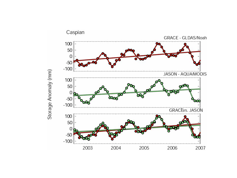
Two ways of estimating Caspian Sea mass change: (1)GRACE minus GLDAS (2) Jason sea surface height minus steric sea level contribution (assume a mixed-layer depth of 28 m).
GRACE minus GLDAS (2) Jason sea surface height minus steric sea level contribution (assume a mixed-layer depth of 28 m).")
16
Greenland Velicogna and Wahr, Nature, 2007

17
Things we do to the GRACE Stokes coefficients to extract the Greenland signal 1.Truncate to a finite harmonic degree. 2.Use a smooth Greenland averaging function. (We do not de-stripe.)
.")
18
Estimating Greenland mass from GRACE G l = smoothing function Finite degree

19
The equivalent spatial averaging functions Exact Greenland average.Truncated averageTruncated and smoothed

20
Extended spatial averaging functions Exact average.Truncated and smoothed

21
Scaling Factors. Estimated from simulated GRACE coeffcients. Truncated and smoothed Spread a uniform 1.0 cm layer of ice over all Greenland. The GRACE averaging function returns an average thickness of 0.54 cm, over the extended area. So multiply the real GRACE estimate by 1.0/0.54 = 1.85. Distribute this same amount of ice uniformly around only the edges of Greenland. The GRACE averaging function returns an average thickness of 0.51 cm. So multiply the real GRACE estimate by 1.0/0.51 = 1.95. We prefer this number

22
Summary When we do things to the Stokes coefficients to reduce noise, we also reduce the signal. To recover an unbiased signal, we need to multiply the monthly signal estimates by a scale factor. To determine the scale factor, we apply our GRACE averaging method to simulated data. When using GRACE to recover a mass signal in an isolated region: The situation is more complicated if the region is not isolated (e.g. the Mississippi River basin).
..")
Similar presentations


 of Level-2 monthly GRACE data Frédéric Frappart 1, Guillaume Ramillien 1, Inga Bergmann.>")


 Understanding Sea-level Rise and Variability 6-9 June, 2006 Paris,>")


