1. Probabilistic & Statistical Techniques Eng. Tamer Eshtawi First Semester 2007-2008 Eng. Tamer Eshtawi First Semester 2007-2008

2. Lecture 13 Chapter 10 (part 2) Correlation and Regression Main Reference: Pearson Education, Inc Publishing as Pearson Addison-Wesley.

3. Section 10-3 Regression

4. Key Concept The key concept of this section is to describe the relationship between two variables by finding the graph and the equation of the straight line that best represents the relationship. The straight line is called a regression line and its equation is called the regression equation.

5. Regression y = mx + b y = b 0 + b 1 x b 0 b 1 The typical equation of a straight line y = mx + b is expressed in the form y = b 0 + b 1 x, where b 0 is the y -intercept and b 1 is the slope. x y The regression equation expresses a relationship between x (called the independent variable, predictor variable or explanatory variable), and y (called the dependent variable or response variable). ^

6. Requirements 1. The sample of paired ( x, y ) data is a random sample of quantitative data. 2. Visual examination of the scatter plot shows that the points approximate a straight-line pattern. 3. Any outliers must be removed if they are known to be errors. Consider the effects of any outliers that are not known errors.

7. Definitions  Regression Equation Given a collection of paired data, the regression equation  Regression Line The graph of the regression equation is called the regression line (or line of best fit, or least squares line). algebraically describes the relationship between the two variables.

8. Regression

9. Notation for Regression Equation Y - intercept of regression equation  0 b 0 Slope of regression equation  1 b 1 Equation of the regression line Population Parameter Sample Statistic

10. Formulas for b 0 and b 1 The regression line fits the sample points best.

11. Example 1 Using the simple random sample of data below, find the value of r. In the last lecture, we used these values to find that the linear correlation coefficient of r = –0.956. Use this sample to find the regression equation.

12. Calculating the Regression Equation - cont

13. Calculating the Regression Equation - cont The estimated equation of the regression line is:

14. Example 2 given find the regression equation.

16. In predicting a value of y based on some given value of x... 1. If there is not a linear correlation, the best predicted y -value is y. Predictions 2.If there is a linear correlation, the best predicted y -value is found by substituting the x -value into the regression equation.

17. From a previous example, we found that the regression equation is y = 34.8 + 0.234 x, ( r = 0.926). Assuming that x = 180 sec, find the best predicted value of y Example 3 We must consider whether there is a linear correlation that justifies the use of that equation. We do have a significant linear correlation (with r = 0.926).

18. 1. If there is no linear correlation, don’t use the regression equation to make predictions. 2. A regression equation based on old data is not necessarily valid now. 3. Don’t make predictions about a population that is different from the population from which the sample data were drawn. Guidelines for Using The Regression Equation

19. Definitions  Marginal Change The marginal change is the amount that a variable changes when the other variable changes by exactly one unit.  Outlier An outlier is a point lying far away from the other data points.  Influential Point An influential point strongly affects the graph of the regression line.

20. Residual The residual for a sample of paired ( x, y ) data, is the difference ( y - y ) between an observed sample y -value and the value of y, which is the value of y that is predicted by using the regression equation. ^ Definition residual = observed y – predicted y = y - y ^

21. Linear regression with small residual error Linear regression with large residual error

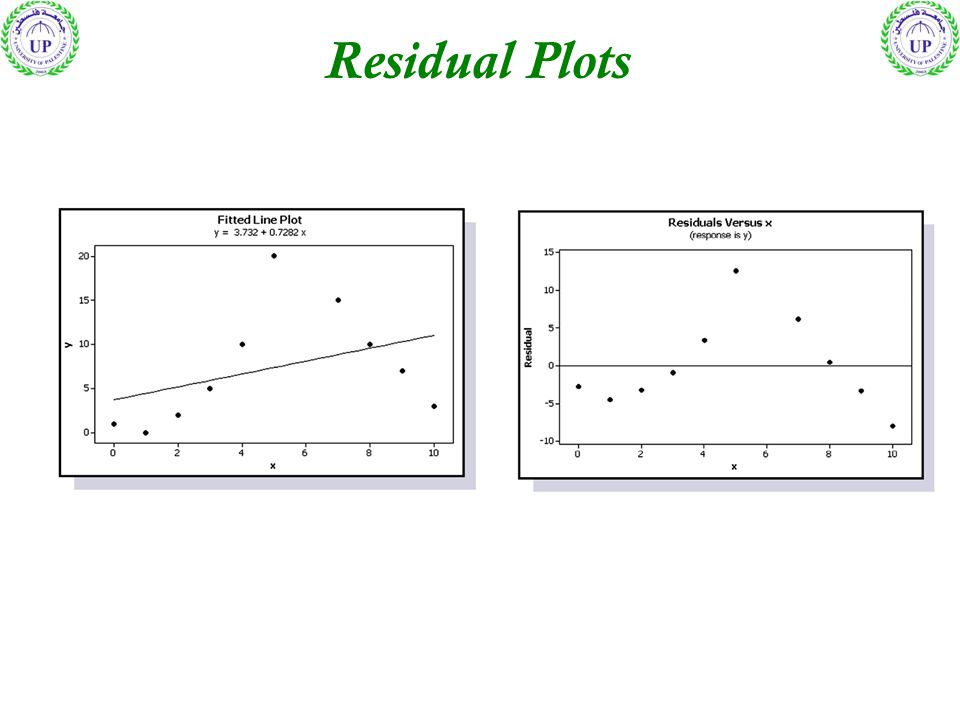
22.  Least-Squares Property A straight line has the least-squares property if the sum of the squares of the residuals is the smallest sum possible.  Residual Plot A scatter plot of the ( x, y ) values after each of the y - coordinate values have been replaced by the residual value. That is, a residual plot is a graph of the points ( x, ) Definitions

23. Residual Plot Analysis  If a residual plot does not reveal any pattern, the regression equation is a good representation of the association between the two variables.  If a residual plot reveals some systematic pattern, the regression equation is not a good representation of the association between the two variables.

24. Residual Plots

27. Section 10-4 Variation and Prediction Intervals

28. Key Concept In this section we proceed to consider a method for constructing a prediction interval, which is an interval estimate of a predicted value of y.

29. Unexplained, Explained, and Total Deviation

30. Definition Total Deviation The total deviation of ( x, y ) is the vertical distance, which is the distance between the point ( x, y ) and the horizontal line passing through the sample mean y.

31. Definition Explained Deviation The explained deviation is the vertical distance, which is the distance between the predicted y - value and the horizontal line passing through the sample mean y.

32. Definition Unexplained Deviation The unexplained deviation is the vertical distance which is the vertical distance between the point ( x, y ) and the regression line. (The distance is also called a residual).

33. (total deviation) = (explained deviation) + (unexplained deviation) Relationships (total variation) = (explained variation) + (unexplained variation)

34. Definition r2 =r2 = Explained variation. Total variation The value of r 2 is the proportion of the variation in y that is explained by the linear relationship between x and y. Coefficient of determination r 2 is the amount of the variation in y that is explained by the regression line.

35. Standard Error of Estimate The standard error of estimate, denoted by S e is a measure of the differences (or distances) between the observed sample y -values and the predicted values y that are obtained using the regression equation. Definition ^

36. Standard Error of Estimate or

37. find the standard error S e based on the following: Given: n = 8  y 2 = 60,204  y = 688  xy = 154,378 b 0 = 34.7698041 b 1 = 0.2340614319 Example:

38. Example (a) Calculate the least squares estimates of the slope and intercept. (b) Use the equation of the fitted line to predict what pavement deflection would be observed when the surface temperature is 85F. (c) Determine the standard error Regression methods were used to analyze the data from a study investigating the relationship between roadway surface temperature ( x ) and pavement deflection ( y ). Summary quantities were

39. (a) Calculate the least squares estimates of the slope and intercept.

40. (c) Determine the standard error (b) Use the equation of the fitted line to predict what pavement deflection would be observed when the surface temperature is 85 F.